Week 3 - Solving second order ODEs

clear all
close all
clc

b = 0.05;
g = 9.81;
l = 1;
m = 1;

%initial conditions (position & velocity)
theta_0 = [0;3];

%time points
t_span = linspace(0,20,250);

%solving ODE
[t,results] = ode45(@(t,theta) ode_func(t,theta,b,g,l,m),t_span,theta_0);

%graph
figure(1)
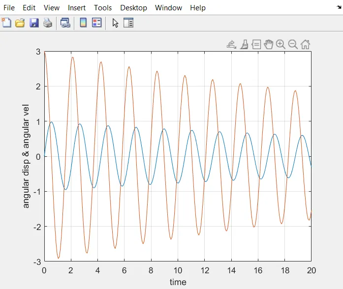
plot(t,results(:,1))
hold on
plot(t,results(:,2))
xlabel('time')
ylabel('angular disp & angular vel')
grid on 

%animation
figure(2)
ct =1;
for i = 1:length(t_span)
    x0 = 0;
    y0 = 0;
    x1 = l*sind(results(i,1));
    y1 = -l*cosd(results(i,1));
    plot([x0 x1],[y0 y1],[-0.5 0.5],[0 0],'linewidth',2)
    hold on
    plot(x1,y1,'marker','o','markerSize',20,'markerFacecolor','c')
    axis([-0.1 0.1 -1.5 0.5])
    pause(0.001)
    M(ct) = getframe(gcf);
    ct = ct+1;
    hold off
end

movie(M)
videofile = VideoWriter('PendulumSwing.avi','Uncompressed AVI')
open(videofile)
writeVideo(videofile,M)
close(videofile)

ODE Function

function [dtheta_dt] = ode_func(t, theta, b, g, l, m)

theta1 = theta(1);
theta2 = theta(2);
dtheta1_dt = theta2;
dtheta2_dt = -(b/m)*theta2-(g/l)*sin(theta1);
dtheta_dt = [dtheta1_dt; dtheta2_dt]
end

Steps-

• Declaring input values (b,g,m,l)
• Initial conditions of pendulum set (0;3 - initial position;initial velocity)
• Simulation run-time is 20 as given and creating an array of 250 values
• [t,results] has the results that are to be plot
• ode45 function (in built function) used to solve the DE.
• plot command used to plot (fig 1)
• used 'for' loop to create every frame
• ct command helps 'for' command in going to next frame
• 'movie' command used to create animation

time vs angular displacement & angular velocity graph fig1

video link - https://drive.google.com/file/d/1cjp8QgYyzTs0Y-KzGkRO6DWxrs78trk0/view?usp=sharing