Week 4.1 - Genetic Algorithm

Aim:
To optimise the stalagmite function and find the global maxima of the function.

Objective:
1.To describe the process and concept of Genetic algorithm.
2.To describe and explain syntax of Genetic algorithm in matlab.
3.Plot the graph for F maximum and no.of iteration and all studies.

Introduction to Genetic Algorithm:
1.The Genetic Algorithm experiment is created by charles darwin's theory of Natural evaluation.
2.It is used to create high accurate solution to opimization and the research Nads by Biologival manner which is
a)Mutuation
b)Crossover
c)Selection

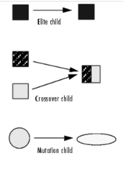
3.It is also used to solve contrained optimization problems and unconstrained optimization problems.

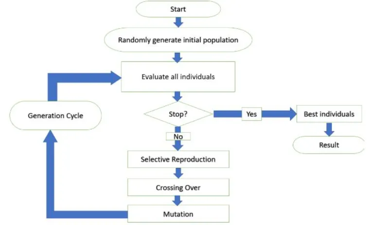
Process of Genetic Algorithm:
1.Coding
2.Fitness function

It defines about the individual how fit to the process, it can also have individual fitness score , based on the score the individuals are taken
3.Selection

selection is the proces of select the fittest part of individual and upgrade them and their genes to produce the next generation the selection is based on two individual which is healthy to make another

4.Reproduction
a)Crossover
b)Mutation

Advantages of Genetic Algorithm:
1.It is Globally optimizable.
2.It Does not more information.
3.It Generates more optimal solution.
4.It is Rapid and Accurate when compared to old method.
Disadvantages:
1.Even though it needs less information the Generation of function and getting correct opration is difficult.
2.The GA is stochastic.
3.Computationally expensive.
Application:
1.It is used in the machine learing process.
2.It is used for DNA sample Analysis.
3.Optimization problem the Genetic Algorithms are commonly used.
4.It is also used in the econimal field.
Syntax for Genetic Algorithm in matlab function:
X=ga(fun,nvars,A,b,Aeq,Beq,lb,ub,nonicon,options)
1.X is the local minimum point.
2.fun it is for the function to be called.
3.nvars- It is for the number of variables used.
4.lb- lower bound.
5.ub- upper bound.
6.A,b- It is linear inequality constraints.
7.Aeq,Beq- It is linear equality contraints.
8.nonicon- It represents the Both inqualilities and equalities.
9.options- To fix the size of the population and customize the options.

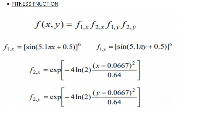
Fitness equations:

coding :

1.The function coding is created and which is stalagmite function and it so

%the function program should be created and named as stalagmitefunc
function[f]=stalagmitefunc(input_vector)
%create the program for assigning the input
x=input_vector(1);
y=input_vector(2);
%for calculating the stalagmite fitness function is used
%the function as (f1_x*f2_x*f1_y*f2_y)
f1_x=(sin(5.1*pi*x+0.5)).^6;
f1_y=(sin(5.1*pi*y+0.5)).^6;
t1=((x-0.0667).^2)/(0.64);
f2_x=exp(-4.*log(2)*t1);
t2=((y-0.0667).^2)/(0.64);
f2_y=exp(-4.*log(2)*t2);
%all these fx and fy values are multiplied to get f
f=-(f1_x.*f2_x.*f1_y.*f2_y);
end

2.The 1st iteration coding is created which has unbounded inputs

clear
close all
clc
%create the input values in the use of of the linspace command
x=linspace(0,0.6,150);
y=linspace(0,0.6,150);
%create the matrix with use of meshgrid command
[xx,yy]=meshgrid(x,y);
%number of iteration for the function evaluation
num_cases=50;
%for creating the surface plot of the stalagmite function
%the for loop will be created in terms i and j
for i=1:length(xx)
for j=1:length(yy)
input_vector(1)=xx(i,j);
input_vector(2)=yy(i,j);
f(i,j)=stalagmitefunc(input_vector);
end
end
%calculating the time with the use of tic command
tic
%an another for loop will be created
%it is for calculating the optimized value of the function
for i=1:num_cases
[input,fopt(i)]=ga(@stalagmitefunc,2);
xopt(i)=input(1);
yopt(i)=input(2);
end
%display the timetaken as the output
study1_time=toc
%plotting the graph
subplot(2,1,1)
%the graph is created as surface
surfc(xx,yy,-f);
hold on
%the shading interp command is used for smooth transition colour
%and hide the grids
shading interp
%the bounds will be created by using marker and 'o' command
plot3(xopt,yopt,-fopt,'marker','o','markersize',5,'markerfacecolor','r');
%naming the axis as x and y
xlabel('x');
ylabel('y');
grid on
subplot(2,1,2)
plot(-fopt);
% the title will be named as un bounded output
title('unbounded inputs')
xlabel('number of iterations');
ylabel('function max');

3. The 2nd iteration is created which has bounded inputs

clear
close all
clc
%create the input values in the use of of the linspace command
x=linspace(0,0.6,150);
y=linspace(0,0.6,150);
%create the matrix with use of meshgrid command
[xx,yy]=meshgrid(x,y)
%for creating the surface plot of the stalagmite function
%the for loop will be created in terms i and j
for i=1:length(xx)
for j=1:length(yy)
input_vector(1)=xx(i,j);
input_vector(2)=yy(i,j);
f(i,j)=stalagmitefunc(input_vector);
end
end
%number of iteration for the function evaluation
num_cases=100;
%calculating the time with the use of tic command
tic
%an another for loop will be created
%it is for calculating the optimized value of the function
for i=1:num_cases
[input,fopt(i)]=ga(@stalagmitefunc,2,[],[],[],[],[0,0],[0.6,0.6]);
xopt(i)=input(1);
yopt(i)=input(2);

end
%display the timetaken as the output
study2_time=toc
%plotting
subplot(2,1,1)
hold on
%plotting it as surface
surfc(xx,yy,-f)
%the shading interp command is used for smooth transition colour
%and hide the grids
shading interp
%the bounds will be created by using marker and 'o' command
plot3(xopt,yopt,-fopt,'marker','o','markersize',5,'markerfacecolor','r')
%assigning tghe title
title('bounded inputs')
%naming the axis
xlabel('x');
ylabel('y');
grid on
subplot(2,1,2)
plot(-fopt);
xlabel('iterations')
ylabel('function min value')

4. The 3rd iteration is created which incresed in population size method

clear all
close all
clc
%create the input values in the use of of the linspace command
x=linspace(0,0.6,150);
y=linspace(0,0.6,150);
%create the matrix with use of meshgrid command
[xx,yy]=meshgrid(x,y);
%for creating the surface plot of the stalagmite function
%the for loop will be created in terms i and j
for i=1:length(xx)
for j=1:length(yy)
input_vector(1)=xx(i,j);
input_vector(2)=yy(i,j);
f(i,j)=stalagmitefunc(input_vector);
end
end
%number of iteration for the function evaluation
num_cases=150;
%this section the population will be altered
%by use population size
options=optimoptions('ga');
options=optimoptions(options,'populationsize',450)
%calculating the time with the use of tic command
tic
%an another for loop will be created
%it is for calculating the optimized value of the function
for i=1:num_cases
[input,fopt(i)]=ga(@stalagmitefunc,2,[],[],[],[],[0;0],[1;1],[],[],options);
xopt(i)=input(1);
yopt(i)=input(2);
end
%display the timetaken as the output
study3_time=toc
figure(3)
%plotting
subplot(2,1,1)
hold on
%plotting it as surface
surfc(xx,yy,-f)
%the shading interp command is used for smooth transition colour
%and hide the grids
shading interp
%the bounds will be created by using marker and 'o' command
plot3(xopt,yopt,-fopt,'marker','o','markersize',5,'markerfacecolor','r');
%assigning the title
title('bounded inputs with incresed population size')
%naming the axis
xlabel('x');
ylabel('y');
grid on
subplot(2,1,2)
plot(-fopt);
xlabel('iterations')
ylabel('function min value')

Procedure:
1.At the First process we need to create stalagmite function.For called into main Genetic Algorithm program.
2.Next the Another code is to be created for the iteration.
3.In iteration code we need to define X and Y inputs using the "linespace" command.
4.Using the command "meshgrid" the input variable are converted as array (xx,yy) evaluation and plotting.
5.Create a iteration loops of "i" and then "j" for the function.
6.Create the stalagmite function calling, so the value are formed in matrix.
7.Using "num_cases" command total Number of time for run of GA is defined.
8.In the use of for loop the Ga value stores in Array for each iteration.
9.By using the Negative sign we can get a maxima which is Inverse stalagmite function and the curves are found.
10.By using "tic" and "toc" command the time is and function evaluation and of GA.
11.Then using "plot" command the final results are plotted and using "surf" command also.
12.The Three sparate iteration loop is to be created. one is unbounded and another is bounded and bounded with polpulation method

Errors:

• The small and spelling mistake Error only came like input is writen as inputs
• And small variation in the grapgb due to x and y variation and this errors are rectified by creating the one to one session by support engineer

Result and Discussion:

1st iteration output(unbounded inputs)

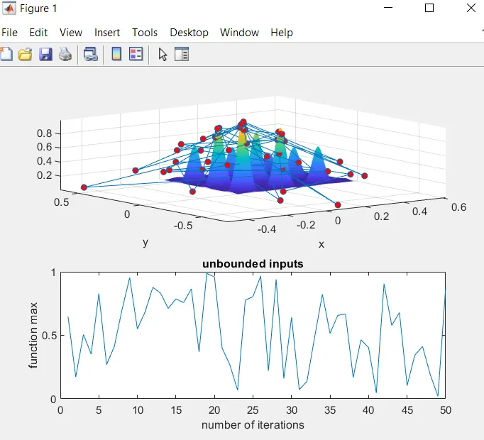
this graph shows that the clumsy output and cant gives any idea and not shows the global maxima so it is not recommened to find ga

2nd iteration output(bounded inputs)

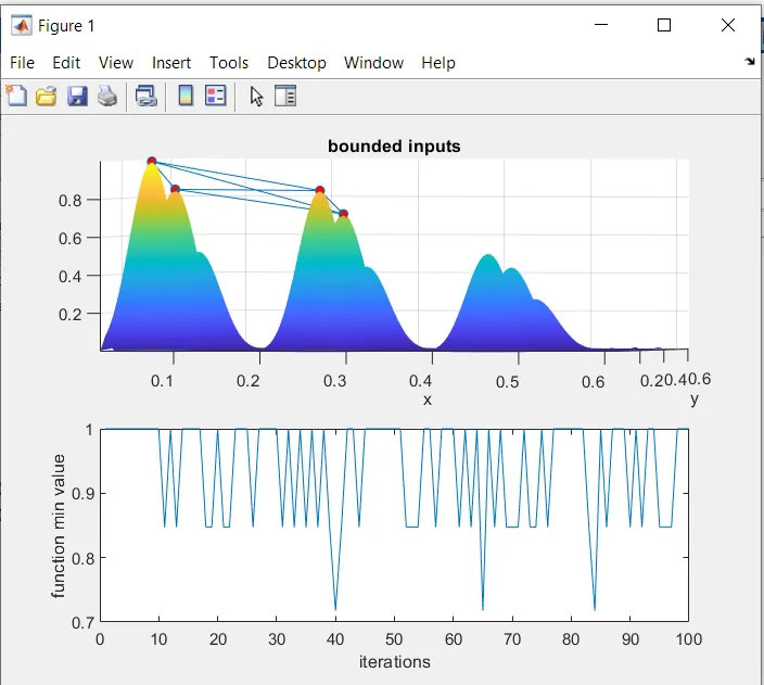
In this study we can observe that the global ,maxima but not clealy comparing the previous one it is ok but not much clear so ifrom this method also global maxima was not clealy observed

3rd iteration output(population method)

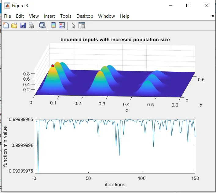
In this method we can observe the global maxima by increase the population size with the bounded inputs so we clearly and exact value of global maxima where noted

so, this study was concluded that comparing the three the population method gives the best value and better results