Challenge

Week 3 - Solving second order ODEs

SSurendhar V11 Apr 2022

MATLAB

AIM:

To create and solve the second order ordinary derivative equation and create a animation using MATLAB

OBJECTIVE:

To write program for solving the below ODE with a graph of velocity v/s displacement with animation

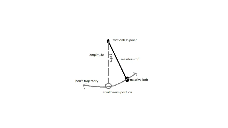
where

g=gravity in m/s^2,

L=lenth of a pendulum in m,

m=mass of the ball in kg

b=damping coefficient

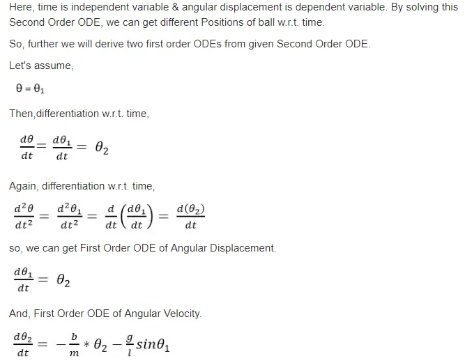
GOVERNING EQUATION:

GIVEN DATA:

L=1 metre

m=1kg

b=0.05

g=9.81 m/s^2

Simulate the motion between 0-20 sec,

for angular displacement=0,

angular velocity=3 rad/sec at time t=0.

CODE:

1. code for function ode 45 for the ode program

%function calling for a ODE and the inputs are the t,thet,b,g,l,m

function [dtheta_dt]=ode_function(t,theta,b,g,l,m)

theta1=theta(1)% assigning the theta 1 ans 2 values

theta2=theta(2)

dtheta1_dt=theta2% diif the theta1= theta 2

dtheta2_dt=-(b/m)*theta2-(g/l)*sin(theta1);%diff of theta 2

dtheta_dt=[dtheta1_dt;dtheta2_dt]

end

this program could saved ode function.m in the same folder where the main code saved it is for the function calling

2.main ode program

clear all

close all

clc

% for per forming this we have to assign the given data as ipt data

l=1; %length of pendulum in metre

m=1;%mass of bob in kg

b=0.05;% damping coeff

g=9.81;% gravity in m/s^2

% initial conditions are

theta_0=0;

omega_0=3;

%time span which is the set of datas which start and end points

t_span=linspace(0,20,500);

% this is the main part of the program solving ODE by function call

[t,results]=ode45(@(t,theta) ode_function(t,theta,b,g,l,m),t_span,[0 3]);

figure(1)

%ploting time and velocity

plot(t,results(:,1));

hold on

plot(t,results(:,2));

xlabel('time')

ylabel('velocity')

%using legend command for identifying each vlues in graph

legend('displacement','Angular velociy');

hold off

disp=results(:,1);

velocity=results(:,2);

%counter at initial

ct=1;

% creating the iteartion loops for accurate statement

for i=1:length(t_span)

%fix the coordinates

x0=0;

y0=0;

%coordinates is calculated as

x1=l*sin(disp(i));

y1=-l*cos(disp(i));

figure(2)

%plotting the fixed link

plot([-2 2],[0 0],'linewidth',5)

hold on

%creating bob using marker command

plot([x0 x1],[y0 y1],'-o','markersize',3,'linewidth',3,'Color','y');

plot(x1,y1,'-o','markersize',15,'markerfacecolor','r');

%setting the axis

axis([-1.5 1.5 -1.5 1.5])

pause(0.03)

hold off

M(ct)=getframe(gcf);

%the counter variable is increased by with loops

ct=ct+1;

end

%creatinyg the animation by using the movie command

movie(M);

%creating the video file and saved in uncompressed AVI formaat

videofile=VideoWriter('pendulum_challenge.avi','Uncompressed AVI')

%opening the video if running the code

open(videofile)

% this for wrtting the video file

writeVideo(videofile,M)

%after the code ends the file closing

close(videofile)

EXPLANATION FOR THE CODE:

1.Initially the given details in the question are aasignned as the inputs and the time is varied and boundary is created by linspace coommand ahge theta valuev is assigned as a column matrix

2.Then the ode45 which is the inbuilt function which is used for function call in program it is set as equal (t,results)

3.Then we use the plot command for plot the graph for the time and velocity and the legend command is used for ideentifying the each values

4.The looping statements is used for the correct and accurate simulation t

5.Next we have to assign the fixed coordinates (x0=1,y0=1,ct=1)

6.For getting the bob in the animation we use the marker command

7. The use of the axis command axis are fixed(axis([0 2 -0.5 2]))

8. the counter variable which ct is used and its value also changed for each loop(ct=ct+1)

9.next we have to create a movie for that so we need to create a videofile and saved in AVI file with compressed format

10. And then add the title for the video

RESULTS:

OUTPUTS-

1. graph for velocity and time and it shows the displacement and angular velocity

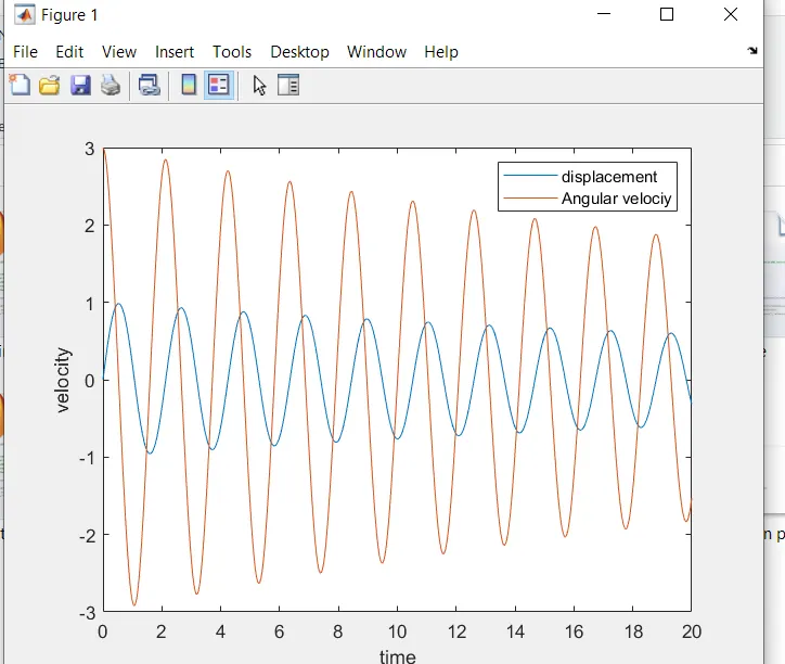
this above graph shows that displacement and velocity is decreasing while time is increasing because of the damper(the damper that absorbs the vibration for body kept in equilibirium position)

2.Animation

https://youtu.be/bvNlxKWBqKo

ERRORS:

1. small mistake has been made bytyping which is used this \ symbol instesd of this /

2.another mistake is assigning in nthe function calling program

this rectified by the experts through one to one sessions

CONCLUSION:

1. the graph for velocity and time is obtained

2. the animation also created and uploaded

Week 3 - Solving second order ODEs

Ship work like this
in your own course.

Talk to a career counsellor

Ship work like thisin your own course.

Talk to a career counsellor

Ship work like this
in your own course.