AIM:-

TO solve a program for stalagmite model for the genetic algorithm by using MATLAB.

OBJECTIVE OF THE PROJECT:-

The main objective of the project is to find the minimum value of the stalagmite function with respective to the number of iteration given as input.the work flow of the project starts with creating 2dimensional mesh where one dimensional array are created with help of 1D array the 2D is created folllowing the flow the stalagmite function is evaluated,for X&Y were we basically creating an array called input. the stalagmite takes the input and calculated the f.by using the given foemulas in the question the coding for stalagmite funtion is to be done to get minimum value of stalagmite function with different case study to make 3D graph for genetic algorithm.

BASIC CONCEPTS:-

OPTIMIZATION:-

Optimization is an area of the study which is used to maximize (or) minimize the particular function,which depends upon multiple parameters to get the desired output.

STALAGMITE MATHEMATICAL MODEL:-

Stalagmite mathematical model is used to develop the local maxima (or) minima.here to determine the optimum solution of the maxima of the function we are using the genetic algorithm technique. the explanation of the genetic algorithm is follows.

GENETIC ALGORITHM:-

Nature has always been a great source of inspiration to all mankind. Genetic Algorithms (GAs) are search based algorithms based on the concepts of natural selection and genetics. GAs are a subset of a much larger branch of computation known as Evolutionary Computation.

GAs were developed by John Holland and his students and colleagues at the University of Michigan, most notably David E. Goldberg and has since been tried on various optimization problems with a high degree of success.

In GAs, we have a pool or a population of possible solutions to the given problem. These solutions then undergo recombination and mutation (like in natural genetics), producing new children, and the process is repeated over various generations. Each individual (or candidate solution) is assigned a fitness value (based on its objective function value) and the fitter individuals are given a higher chance to mate and yield more “fitter” individuals. This is in line with the Darwinian Theory of “Survival of the Fittest”.

In this way we keep “evolving” better individuals or solutions over generations, till we reach a stopping criterion.

Genetic Algorithms are sufficiently randomized in nature, but they perform much better than random local search (in which we just try various random solutions, keeping track of the best so far), as they exploit historical information as well.

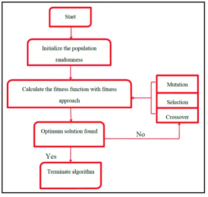
Selection

The idea of selection phase is to select the fittest individuals and let them pass their genes to the next generation.

Two pairs of individuals (parents) are selected based on their fitness scores. Individuals with high fitness have more chance to be selected for reproduction.

Crossover

Crossover is the most significant phase in a genetic algorithm. For each pair of parents to be mated, a crossover point is chosen at random from within the genes.

For example, consider the crossover point to be 3 as shown below.

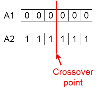
Crossover point

Offspring are created by exchanging the genes of parents among themselves until the crossover point is reached.

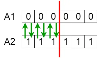
Exchanging genes among parents

The new offspring are added to the population.

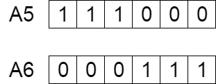
New offspring

Mutation

In certain new offspring formed, some of their genes can be subjected to a mutation with a low random probability. This implies that some of the bits in the bit string can be flipped.

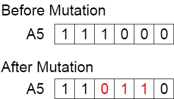
Mutation: Before and After

Mutation occurs to maintain diversity within the population and prevent premature convergence.

Function(1):

Fitness Function

The fitness function determines how fit an individual is (the ability of an individual to compete with other individuals). It gives a fitness score to each individual. The probability that an individual will be selected for reproduction is based on its fitness score.

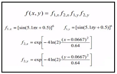
And now we are writing the stalagmite function based on the above formula is as,

%stalagmite function

function sol = stalagmite(input)
x = input(1);
y = input(2);
fxone = (sin(((5.1*pi).*x)+0.5)).^6;
fxtwo = exp((((x-0.0667).^2).*(-4*log(2)))./0.64);
fyone = (sin(((5.1*pi).*y)+0.5)).^6;
fytwo = exp((((y-0.0667).^2).*(-4*log(2)))./0.64);
sol = -((fxone)*(fxtwo)*(fyone)*(fytwo));
end

Function(2):

The new function is containing the for loop command and mesh grip command only.here we are not using the one demensional array x and y with the linspace command.because the x and y are the input array not define the workspace for the genetic algorithm.hence it is unnecessary in this function.

[xx yy] = meshgrid(x,y);

%evaluating stalagmite function
for i = 1:length(xx)
    for j = 1:length(yy)
        input(1)=xx(i,j);
        input(2)=yy(i,j);
        f(i,j) = stalagmite(input);
    end
end

SYNTAX REFERRED FOR GRNRTIC ALORITHM:-

In the main program we are going to use the one dimensional array x and y with linspace command and as we know the x and y are input array it does not define the workspace for the genetic algorithm.

the syntax use for the genetic algorithm is as shown below

Syntax

x = ga(fun,nvars)

x = ga(fun,nvars,A,b)

x = ga(fun,nvars,A,b,Aeq,beq)

x = ga(fun,nvars,A,b,Aeq,beq,lb,ub)

x = ga(fun,nvars,A,b,Aeq,beq,lb,ub,nonlcon)

x = ga(fun,nvars,A,b,Aeq,beq,lb,ub,nonlcon,options)

x = ga(fun,nvars,A,b,[],[],lb,ub,nonlcon,IntCon)

x = ga(fun,nvars,A,b,[],[],lb,ub,nonlcon,IntCon,options)

x = ga(problem)

[x,fval] = ga(___)

[x,fval,exitflag,output] = ga(___)

[x,fval,exitflag,output,population,scores] = ga(___)

WHERE:-

x = ga(fun,nvars,A,b) finds a local minimum x to fun, subject to the linear inequalities A*x ≤ b. ga evaluates the matrix product A*x as if x is transposed (A*x').

x = ga(fun,nvars,A,b,Aeq,beq) finds a local minimum x to fun, subject to the linear equalities Aeq*x = beq and A*x ≤ b. (Set A=[] and b=[] if no linear inequalities exist.) ga evaluates the matrix product Aeq*x as if x is transposed (Aeq*x').

x = ga(fun,nvars,A,b,Aeq,beq,lb,ub) defines a set of lower and upper bounds on the design variables, x, so that a solution is found in the range lb ≤ x ≤ ub. (Set Aeq=[] and beq=[] if no linear equalities exist.)

x = ga(fun,nvars,A,b,Aeq,beq,lb,ub,nonlcon) subjects the minimization to the constraints defined in nonlcon. The function nonlcon accepts x and returns vectors C and Ceq, representing the nonlinear inequalities and equalities respectively. ga minimizes the fun such that C(x) ≤ 0 and Ceq(x) = 0. (Set lb=[] and ub=[] if no bounds exist.)

x =ga(fun,nvars,A,b,Aeq,beq,lb,ub,nonlcon,options) minimizes with the default optimization parameters replaced by values in options. (Set nonlcon=[] if no nonlinear constraints exist.) Create options using optimoptions.

x = ga(fun,nvars,A,b,[],[],lb,ub,nonlcon,IntCon) or x = ga(fun,nvars,A,b,[],[],lb,ub,nonlcon,IntCon,options) requires that the variables listed in IntCon take integer values.

x = ga(problem) finds the minimum for problem, a structure described in problem.

[x,fval] = ga(___), for any previous input arguments, also returns fval, the value of the fitness function at x.

[x,fval,exitflag,output] = ga(___) also returns exitflag, an integer identifying the reason the algorithm terminated, and output, a structure that contains output from each generation and other information about the performance of the algorithm.

[x,fval,exitflag,output,population,scores] = ga(___) also returns a matrix population, whose rows are the final population, and a vector scores, the scores of the final population.

WRITING PROGRAM WITH DIFFERENT OPTIMIZATION STUDEIS:-

clear all
close all
clc

x = linspace(0,0.6,150);
y = linspace(0,0.6,150);
num_cases = 60
[xx yy] = meshgrid(x,y);

%evaluating stalagmite function
for i = 1:length(xx)
    for j = 1:length(yy)
        input(1)=xx(i,j);
        input(2)=yy(i,j);
        f(i,j) = stalagmite(input);
    end
end
tic
% study1-satistical behaviour
for i = 1:num_cases
    [inputs,fopt(i)]=ga(@stalagmite,2);
    xopt(i) = inputs(1);
    yopt(i) = inputs(2);
end

study1_time=toc
figure(1)
subplot(2,1,1)
hold on
surfc(xx,yy,-f)
shading interp
plot3(xopt,yopt,-fopt,'color','b','marker','o','markersize',5,'markerfacecolor','r')
title('unbounded inputs');
subplot(2,1,2)
plot(-fopt,'color','b','linewidth',1)
xlabel('iteration');
ylabel('function minimum');


tic
%study2 statistical behaviour with upper ans lower bonds
for i = 1:num_cases
    [inputs,fopt(i)]=ga(@stalagmite,2,[],[],[],[],[0:0],[1:1]);
    xopt(i) = inputs(1);
    yopt(i) = inputs(2);
end

study2_time=toc
figure(2)
subplot(2,1,1)
hold on
surfc(xx,yy,-f)
shading interp
plot3(xopt,yopt,-fopt,'marker','o','markersize',5,'markerfacecolor','r')
title('bounded inputs')
subplot(2,1,2)
plot(-fopt','color','b','linewidth',1)
xlabel('iteration');
ylabel('function minimum');

%study 3 increasing ga iterations
options = optimoptions('ga');
options = optimoptions(options,'populationsize',800);
tic
for i = 1:num_cases
    [inputs,fopt(i)]=ga(@stalagmite,2,[],[],[],[],[0:0],[1:1],[],[],options);
    xopt(i) = inputs(1);
    yopt(i) = inputs(2);
end
study3_time=toc
figure(3)
subplot(2,1,1)
hold on
surfc(xx,yy,-f)
shading interp
plot3(xopt,yopt,-fopt,'marker','o','markersize',5,'markerfacecolor','r')
title('bounded inputs with increasing ga')
subplot(2,1,2)
plot(-fopt)
xlabel('iteration');
ylabel('function minimum');

EXPLANATION FOR STUDY (1)

*x=linspace(0,0.6,150):-linspace command is used for providing intervals with a given value,where the value for x and y is given and these are the input array of x and y.

*y=linspace(0,0.6,150):-linspace command is used for providing intervals with a given value,where the value for x and y is given and these are the input array of x and y.

*num_cases=60:-num cases is 60 called the genetic algorithm to run for 60 times.

*[xx,yy]=meshgrid(x,y):- the command is used to mesh the 2d and 3d plot,where x and y are the axis the plots to meshed.

*for i = 1:length(xx) for loop is created for repeating the set of values with respective to x-axis

*for j = 1:length(xx) for loop is created for repeating the set of values with respective to y-axis

*input(1)=xx(i,j):-for each value of x basically an array created called input.

*input(2)=yy(i,j):-for each value of y basically an array created called input

*f(i,j)=stalagmite(input):where stalagmite is a function.the stalagmite takes the input and calculated the f.

*end- the command must be use when the loop is called.

*tic-the command is used to calculate the operation time performed.

*[input,fopt(i)]=ga(@stalagmite,2,] where the study for the statistical behaviour is started with inputs and fopt(i) are the variables for the given input.stalagmite is a function a code is written seperately and called for the operation.2 is the no of variable as inputs.

*xopt(i)=input(1):-the x value for the inputs in written with the variable called xopt.

*yopt(i)=input(2):-the y value for the inputs in written with the variable called yopt.

*end:-forloop is called so end must be used.

*study1_time-toc:-the command is used to calculate the operation time performed for study 1.

*subplot(2,1,1)-the sub plot command is used to creating multiple plot.the 2,1 is the x and y axis with respective to first column.

*hold on-the command is used for adding new elements for showing the graph.

*surfc(xx,yy,-f)-surfc command is used for creating the surface for the function.

*shading interp-the command is used to plot the 3d graph were the grid on the 3d will be as smooth shading.
*plot3(xopt,yopt,-fopt,'color','b','marker','o','markersize',5,'markerfacecolor','r') the command is used for plottting the x,y,z axis in the graph.the marker and markersize command are used to created the sizee and shape of the maxima.

*title('unbounded inputs');-the command is used to represent the graph name.

*subplot(2,1,2)-the subplot command is used to creating multiple plot with a plotr.the 2,1 is the x and y axis with the respective to second column.

*plot(-fopt,'color','b','linewidth',1) -is given to plot the graph is maxima.

*xlabel('iteration');-xlabel is the command used for creating x-axis name.

*ylabel('function minimum');=ylabel is the command used for creating y-axis name.

Graph for study 1:-

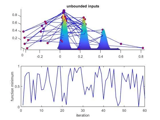
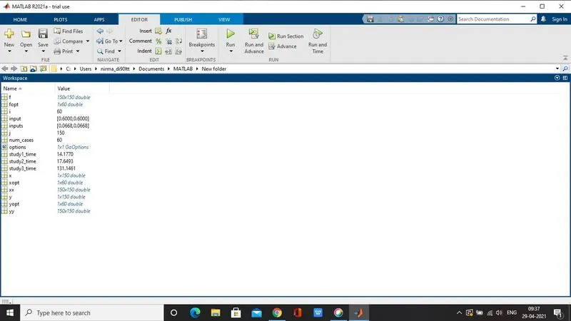
STUDY1_TIME=14.1770

EXPLANATION OF STUDY 2:-

*tic-the command is used to calculate the operation time performed.

*[input,fopt(i)]=ga(@stalagmite,2,[],[],[],[],[0:0],[1:1])] where the study for the statistical behaviour is started with inputs and fopt(i) are the variables for the given input.stalagmite is a function a code is written seperately and called for the operation.2 is the no of variable as inputs,[],[],[],[],ARE THE VARIABLE ARGUMENTS.[0:0],[1:1] are the xx and yy .

*xopt(i)=input(1):-the x value for the inputs in written with the variable called xopt.

*yopt(i)=input(2):-the y value for the inputs in written with the variable called yopt.

*end:-forloop is called so end must be used.

*study2_time-toc:-the command is used to calculate the operation time performed for study 2.

*subplot(2,1,1)-the sub plot command is used to creating multiple plot.the 2,1 is the x and y axis with respective to first column.

*hold on-the command is used for adding new elements for showing the graph.

*surfc(xx,yy,-f)-surfc command is used for creating the surface for the function.

*shading interp-the command is used to plot the 3d graph were the grid on the 3d will be as smooth shading.

*plot3(xopt,yopt,-fopt,'color','b','marker','o','markersize',5,'markerfacecolor','r') the command is used for plottting the x,y,z axis in the graph.the marker and markersize command are used to created the sizee and shape of the maxima.

*title('bounded inputs');-the command is used to represent the graph name.

*subplot(2,1,2)-the subplot command is used to creating multiple plot with a plotr.the 2,1 is the x and y axis with the respective to second column.

*plot(-fopt,'color','b','linewidth',1) -is given to plot the graph is maxima.

*xlabel('iteration'):-xlabel is the command used for creating x-axis name.

*ylabel('function minimum'):-ylabel is the command used for creating y-axis name.

GRAPH FOR STUDY 2 :-

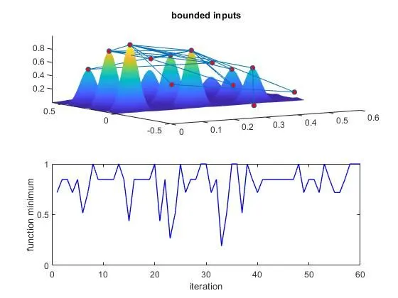
STUDY2_TIME=17.6493

EXPLANATION OF STUDY 3:-

*options=optimopyions('ga');-the command is a solver name were used to solve ga

*options=optimoptions('options,'population',800);the command is a solver name where x,y and the value for the population size is given.

*tic-the command is used to calculate the operation time performed.

*[input,fopt(i)]=ga(@stalagmite,2,[],[],[],[],[0:0],[1:1],[],[],options)] where the study for the statistical behaviour is started with inputs and fopt(i) are the variables for the given input.stalagmite is a function a code is written seperately and called for the operation.2 is the no of variable as inputs,[],[],[],[],ARE THE VARIABLE ARGUMENTS.[0:0],[1:1] are the xx and yy ans the value argument with options solver is used for running function.

*xopt(i)=input(1):-the x value for the inputs in written with the variable called xopt.

*yopt(i)=input(2):-the y value for the inputs in written with the variable called yopt.

*end:-forloop is called so end must be used.

*study3_time-toc:-the command is used to calculate the operation time performed for study 2.

*subplot(2,1,1)-the sub plot command is used to creating multiple plot.the 2,1 is the x and y axis with respective to first column.

*hold on-the command is used for adding new elements for showing the graph.

*surfc(xx,yy,-f)-surfc command is used for creating the surface for the function.

*shading interp-the command is used to plot the 3d graph were the grid on the 3d will be as smooth shading.

*plot3(xopt,yopt,-fopt,'color','b','marker','o','markersize',5,'markerfacecolor','r') the command is used for plottting the x,y,z axis in the graph.the marker and markersize command are used to created the sizee and shape of the maxima.

*title('bounded inputs with increasing ga');-the command is used to represent the graph name.

*subplot(2,1,2)-the subplot command is used to creating multiple plot with a plotr.the 2,1 is the x and y axis with the respective to second column.

*plot(-fopt,'color','b','linewidth',1) -is given to plot the graph is maxima.

*xlabel('iteration'):-xlabel is the command used for creating x-axis name.

*ylabel('function minimum'):-ylabel is the command used for creating y-axis name.

GRAPH FOR STUDY 3 :-

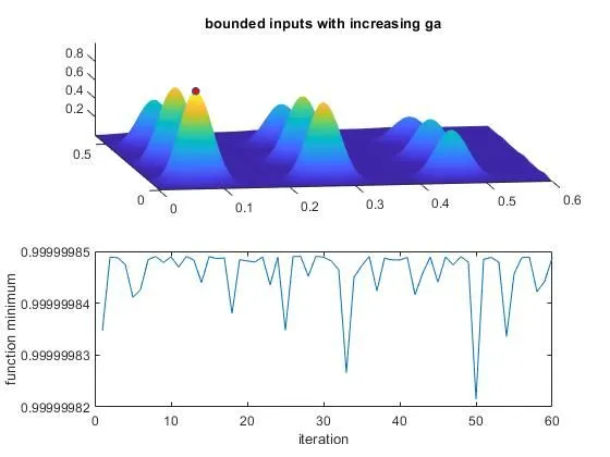
STUDY3_TIME=131.1461

WORKSPACE RESULTS:-