Week 3 - Solving second order ODEs

AIM:-

         To write a program that solves the equation of the motion of a simple pendulum with damping.

THEORY:-

               A second order differential ordinary equation is which any derivatives with respect to the independent variab;le have order no greater than 2.

SIMPLE PENDULUM:-

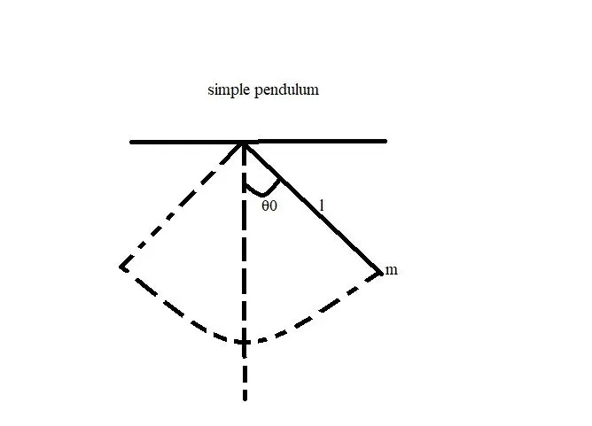
              An ideal pendulum concesisting of a point mass suspended by a weightless inextensible perfectly flexible thread and free to vibrate without friction.

               the way pendulum moves depends on the newton's 2nd law.

OBJECTIVE:-

            To write a program that sloves the following ODE.The ODE represents of motionof a simple pendulum with damping  

In the above equation,

g = gravity in m/s2,

L = length of the pendulum in m,

m = mass of the ball in kg,

b=damping coefficient.

FIXED PARAMETERS:-

LENGTH(l)=1 metre,

MASS(m)=1 kg,

DAMPING COEFFICIENT(b)=0.05.

ACCELERATION DUE TO GRAVITY(g)=9.81 m/s2.

FOR TIME PERIOD= 0-20 sec,

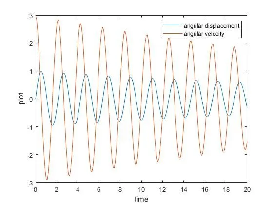
angular displacement=0,angular velocity=3 rad/sec at time t=0.

CODING:-

calling function

function [dtheta_dt] = ode_func(t,theta,b,g,l,m)
theta1 = theta(1)
theta2 = theta(2)
dtheta1_dt = theta2;
dtheta2_dt = -(b/m)*theta2-(g/l)*sin(theta1);
dtheta_dt = [dtheta1_dt;dtheta2_dt];
end

EXPLANATION:-

*In this function program,the scond order ODE is simplified to the first-order ODE by introducing the term theta1 & theta2.

*then theta1 & theta2 is differentiated and the dtheta_dt gives a column matrix.

MAIN PROGRAM:-

% fixed parameters
clear all
close all
clc

b=0.05;
g=9.81;
l=1;
m=1;

%initial condition
theta=[0;3];

%time points
t_span=linspace(0,20,200);
 
[t,results]=ode45(@(t,theta)ode_func(t,theta,b,g,l,m),t_span,theta);

figure(1)
plot(t,results(:,1))
hold on
plot(t,results(:,2))
xlabel('time')
ylabel('plot')
legend('angular displacement','angular velocity')
hold off

ct = 1;
for i= 1:length(t)
    X0 = 0;
    Y0 = 0;
    X1 = 1*sin(results(i,1));
    Y1 = -1*cos(results(i,1));
    
    figure(2)
    plot([X0 X1],[Y0 Y1],'color','r')
    hold on
    plot([1 -1],[0 0],'color','b')
    plot(X1,Y1,'.','markersize',50)
    axis([ -1 1 -1 1 ])
    hold off
    
    M(ct)=getframe(gcf);
    ct=ct+1;
    
end


movie(M)
videofile = VideoWriter('pendulum_ode.avi','Uncompressed AVI');
open(videofile)
writeVideo(videofile,M)
close(videofile)

EXPLANATION:-

*In the above program,the fixed parameters are length,mass,damping coefficient,and acceleration due to gravity.

*time and angle are given as the initial condition.

*in the t_span command,200 values are taken in between 0 to 200 times period.

*using the ode45 command ODE function is introduced.

*using the plot command velocity and displacement is plotted in the y-axis against time in the x-axis.

*using the foor loop command the mass at various points and various times are marked in the graph and are plotted.

*using themovie command the plot is saved as an uncompressed avi file.

PLOT:-