Week 4.1 - Genetic Algorithm

Introduction to optimization:

• Optimization with MATLAB Optimization deals with selecting the best option among a number of possible choices that are feasible or don't violate constraints.

Genetic algorithm-

Genetic Algorithms(GAs) are adaptive heuristic search algorithms that belong to the larger part of evolutionary algorithms. Genetic algorithms are based on the ideas of natural selection and genetics.

These are intelligent exploitation of random search provided with historical data to direct the search into the region of better performance in solution space.

They are commonly used to generate high-quality solutions for optimization problems and search problems.

Advantages-

• The Concept of Genetic algorithm is easy to understand.
• Genetic algorithm is robust with respect to local maxima/minima.
• Genetic algorithm is good for noisy environments.
• The random mutation guarantees in a wide range of solutions.

Disadvantages-

1 GA implementation is still an art.

2 GA requires less information about the problem, but designing an objective function and getting the representation.

3 GA is computationally expensive i.e. time-consuming.

Aim-To write code to calculate global maxima using algorith, using matlab

The stalagmite function is as follows

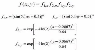
Tha above function is defined in the stalagmite function in matlab as shwon below

function[f]=stalagmite(input_vector) %stalagmite function wih input_vector which contain the x ar

x=input_vector(1);

y=input_vector(2);

f1=(sin(5.1*pi*x+0.5))^6;

f2=(sin(5.1*pi*y+0.5))^6;

f3=exp(-4*log(2)*(x-0.0067)^2/0.64);

f4=exp(-4*log(2)*(y-0.0067)^2/0.64);

f=-(f1*f2*f3*f4)

end

The format for writing genetic algorith in matlab is

x = ga(fun,nvars,A,b,Aeq,beq,lb,ub,nonlcon,intcon,options)

X= minama point

a and b are used to indicate the inequalities that exist in the function

fun-function

Aeq and Beq also denotes the inequalities

nvars denotes no variables used

lb-=lower bound

up-upper bound

1) First iteration:-

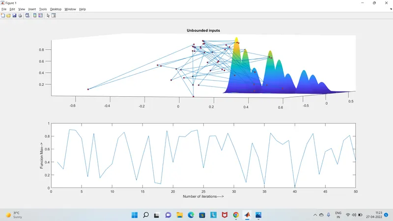
In the first iteration the behaviour of teh algorithm is studied by not defining the limits.

Program-

clear all

close all

clc

num_cases=50 % GA runs for 50 iterations

%defining our search space

x=linspace(0,0.6,150);

y=linspace(0,0.6,150);

%creating a 2D mesh

[xx yy]=meshgrid(x,y);

%evaluating the stalagmite function

for i=1:length(xx)

for j=1:length(yy)

input_vector(1)=xx(i,j);

input_vector(2)=yy(i,j);

f(i,j)=stalagmite(input_vector);

end

end

surfc(x,y,f)

tic % study time count start

for i=1:num_cases

[inputs,f_opt(i)]=ga(@stalagmite,2);

x_opt(i)=inputs(1);

y_opt(i)=inputs(2);

end

f_opt=-f_opt;

study1_time = toc %study time count end

subplot(2,1,1)

hold on

surfc(x,y,-f) % genertaion of stalagmite

shading interp %to bring visually smooth curve witout mesg=hlines

plot3(x_opt,y_opt,f_opt,'marker','o','markersize',4,'markerfacecolor','r')

title('Unbounded inputs')

subplot(2,1,2)

plot(f_opt) % plot of opt_f for every iterations

xlabel('Number of iterations---->')

ylabel('Funcion Max-->')

2) Second iteratio:-

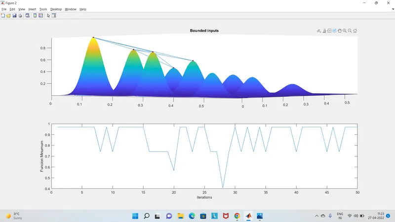
Here the upper and lower bounds are defined soa s to know the boundries within the global maxima lies.

Program-

clear all

close all

clc

num_cases=50 % GA runs for 50 iterations

%defining our search space

x=linspace(0,0.6,150);

y=linspace(0,0.6,150);

%creating a 2D mesh

[xx yy]=meshgrid(x,y);

%evaluating the stalagmite function

for i=1:length(xx)

for j=1:length(yy)

input_vector(1)=xx(i,j);

input_vector(2)=yy(i,j);

f(i,j)=stalagmite(input_vector);

end

end

surfc(x,y,f)

tic % study time count start

for i=1:num_cases

[inputs2,f_opt2(i)]=ga(@stalagmite,2,[],[],[],[],[0 0],[1 1]); %lb of variables of x and Y is (0 0) %ub of variables of x and Y is (1 1)

x_opt2(i)=inputs2(1);

y_opt2(i)=inputs2(2);

end

f_opt2=-f_opt2;

time_study2=toc

figure(2)

subplot(2,1,1)

hold on

surfc(x,y,-f) % genertaion of stalagmite

shading interp %to bring visually smooth curve witout mesg=hlines

plot3(x_opt2,y_opt2,f_opt2,'marker','o','markersize',4,'markerfacecolor','r')

title('Bounded inputs')

subplot(2,1,2)

plot(f_opt2) % plot of opt_f for every iterations

xlabel('iterations')

ylabel('Funcion Minumum')

3) Thrid iteration:-

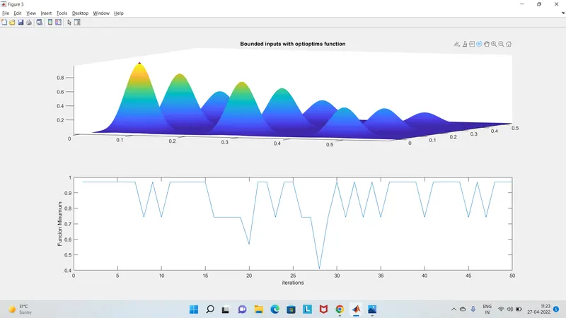
In this itetarion population size is increased as on to converage to the global maxima

Program-

clear all

close all

clc

num_cases=50 % GA runs for 50 iterations

%defining our search space

x=linspace(0,0.6,150);

y=linspace(0,0.6,150);

%creating a 2D mesh

[xx yy]=meshgrid(x,y);

%evaluating the stalagmite function

for i=1:length(xx)

for j=1:length(yy)

input_vector(1)=xx(i,j);

input_vector(2)=yy(i,j);

f(i,j)=stalagmite(input_vector);

end

end

surfc(x,y,f)

options=optimoptions ('ga')

options=optimoptions(options,'PopulationSize',500);

tic % study time count start

for i=1:num_cases

[inputs3,f_opt3(i)]=ga(@stalagmite,2,[],[],[],[],[0 0],[0.6 0.6],[],[],options);

x_opt3(i)=inputs3(1);

y_opt3(i)=inputs3(2);

end

f_opt3=-f_opt3;

figure(3)

subplot(2,1,1)

hold on

surfc(x,y,-f) % genertaion of stalagmite

shading interp %to bring visually smooth curve witout mesg=hlines

plot3(x_opt3,y_opt3,f_opt3,'marker','o','markersize',4,'markerfacecolor','r')

title('Bounded inputs with optioptims function')

subplot(2,1,2)

plot(f_opt2) % plot of opt_f for every iterations

xlabel('iterations')

ylabel('Funcion Minumum')

time_study3=toc

rng('default')

Results

1) First iteration

2) Second iteration

3) Third iteration (population size 500)