Week 4.1 - Genetic Algorithm
OBJECTIVE
The objective of this challenge is to optimize this slagmite function and maximize it using genetic algorithm (ga function) in MATLAB.
Genetic Algorithm
Genetic algorithm is an optimization method based on the biological evolution. The concepts of Natural Selection and Genetic Inheritance are used in this method. This method is used for solving both constrained and unconstrained optimization problems.
The genetic algorithm repeatedly modifies a population of individual solutions. At each step, the genetic algorithm selects individuals at random from the current population to be parents and uses them to produce the children for next generation. Over successive generations, the population evolves toward an aptimal solution.
Working of the Genetic Algorithm
- In the first step algorithm creates a random initial population.
- Second step is to generate sequence of new population by using individuals from current population. The algorithm selects a group of inidviduals in the current population called parents who contribute their genes (the vector elements) to their children.
- Each individual of the current population is scored by computing its fitness value. These vlaues are called the raw fitness scores.
- The raw fitness scores are scaled to convert them into a more usable range of values. These scaled values are called expectation values.
- The algorithm usually selects individuals that have better fitness values as parents.
- By using these parents genetic algorithm creates three types of children for the next generation (elite, crossover and mutation).
- Elite are the individuals in the current generation with the best fitness values. These individuals automatically survive to the next generation.
- Crossover children are created by combining the vectors of a pair of parents.
- Mutation children are created by introducing random changes, or mutations, to a single parent.
- Now the fitness of the new population is determined and the process is repeated to generate new population.
- The algorithm stops when the optimum solution is found.
Syntax for ga in MATLAB
In my program I have used three syntaxes
1) [x, fval] = ga(fun,nvars) - This finds a local unconstrained minimum (x) to the objective function (fun) and also returns the value of fitness function at x.
2) [x, fval] = ga(fun,nvars,A,b,Aeq,beq,lb,ub) - by using this syntax a set of lower and upper bound on the design variables (x) can be defined so that a solution is found in the range ( lb <= x <= ub). (Set Aeq = [] and beq = [] if no linear equality exist.)
3) [x, fval] = ga(fun,nvars,A,b,Aeq,beq,lb,ub,nonlcon,intcon,options) - by using this syntax the objective function is minimized with default optimization parameters replaced by values in options. (Set nonlcon = [] if no non linear constraint exist.) Create options using optimoptions.
| func | Fitness funciton |
| nvars | Number of design variables |
| A | Matrix for linear inequality constraints |
| b | Vector for linear inequality constraints |
| Aeq | Matrix for linear equality constraints |
| beq | Vector for linear equality constraints |
| lb | Lower bound on x |
| ub | Upper bound on x |
| nonlcon | Nonlinear constraint functions |
| intcon | Integer constraint |
| options | Options created using Optimoptions or an options structure |
EXPLANATION OF THE CODE
I've written a function script stalagmite_ga. This will be the objective function which will be maximized using ga in the main script. All the three syntaxes mentioned above will be used in three different cases. I'll will first explain the stalagmite function and then the main script.
User-defined function (stalagmite_ga)
function f = stalagmite_ga(input)

x = input(1);     % initializing the input variable x
y = input(2);     % initializing the input variable y

% mathematical equations for stalagmite function
f_x1 = (sin(5.1*pi*x + 0.5))^6;
f_y1 = (sin(5.1*pi*y + 0.5))^6;
f_x2 = exp(-4*log(2)*(((x - 0.0667)^2)/0.64));
f_y2 = exp(-4*log(2)*(((y - 0.0667)^2)/0.64));

f = -(f_x1*f_x2*f_y1*f_y2);    % note that -ve sign is used here in order to get the maximum value because ga function will by default calculate the minimum value.

end
I've created a function and named it as stalagmite_ga. This function will require one input. The input vector will be 1x2 array. Then the values from the array 'input' are assigned to variables x and y
% Program to optimize the stalagmite function and find the global maxima of the function.
clear
close all
clc

% Defining our search space
x = linspace(0,0.6,150);    % defining search space for x. (150 values between 0 and 0.6)
y = linspace(0,0.6,150);    % defining search space for y. (150 values between 0 and 0.6)
num_cases = 50;             % this variable will be used in the for loop for running the ga function 50 times.

% Creating a 2D mesh
[xx, yy] = meshgrid(x,y);

% Evaluating the stalagmite function
for i = 1:length(xx)                   % initializing the loop variable (i)
    for j = 1:length(yy)               % initializing the loop variable (j)
        input(1) = xx(i,j);            % assigning the values from xx array to first column of variable 'input'
        input(2) = yy(i,j);            % assigning the values from yy array to second column of variable 'input'
        f(i,j) = stalagmite_ga(input); % calling the stalagmite function.
    end
end

f = -f;                                          % this will convert the -ve values returned by stalagmite_ga as output to the positive value. (the stalagmite function (stalagmite_ga) was multiplied with -1)


% Case 1 : Statistical behaviour of GA
tic         % starting the timer
for i = 1:num_cases                              % initializing the for loop variable i.
    [inputs1, fval1(i)] = ga(@stalagmite_ga,2);  % using the ga function to optimize the stalagmite_ga function to its maximum value.
    xopt1(i) = inputs1(1);                       % assigning the returned optimum value of x to xopt1
    yopt1(i) = inputs1(2);                       % assigning the returned optimum value of y to yopt1
end

fval1 = -fval1;                         % this will convert the -ve values returned by ga as output to the positive value. (the stalagmite function (stalagmite_ga) was multiplied with -1)
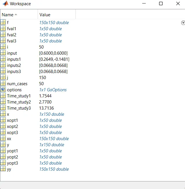
Time_study1 = toc                      % stoping the timer for case 1 and assigning its to variable
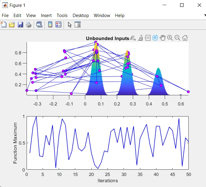
figure(1)                              % figure 1 for case 1
subplot(2,1,1)                         % specifying position for the graph in figure 1
hold on                                % hold on command used to hold the current plot
surfc(x,y,f)                           % using surfc command to plot surface using x, y and f. This command will also draw a contour plot beneath the surface.
shading interp                         % using this command to set shading to interpolated
plot3(xopt1,yopt1,fval1,'color','b','marker','o','markersize',5,'markerfacecolor','m')     % plot3 is used to plot optimum values returned by ga in 3D space
title('Unbounded Inputs');             % title for the plot
subplot(2,1,2)                         % specifying position for the graph in figure 1
plot(fval1,'color','b','linewidth',1)  % plotting fval1
xlabel('Iterations');                  % labelling x-axis
ylabel('Function Maximum');            % labellong y-axis

% Case 2 : Statistical behaviour of GA with specified upper and lower bounds

tic     % Starting the timer
for i = 1: num_cases                                                     % initializing the for loop variable i
    [inputs2, fval2(i)] = ga(@stalagmite_ga,2,[],[],[],[],[0;0],[1,1]);  % by using this syntax I've specified the values of lower bound and upper bound so that the solution if found in the specified range.
    xopt2(i) = inputs2(1);                                               % assigning the returned optimum value of x by ga to xopt2
    yopt2(i) = inputs2(2);                                               % assigning the returned optimum value of y by ga to yopt2
end

fval2 = -fval2;                        % this will convert the -ve values returned by ga for case 2 as output to the positive value. (the stalagmite function (stalagmite_ga) was multiplied with -1)
Time_study2 = toc                      % stopping the counter for case 2 and assigning its value to the variable
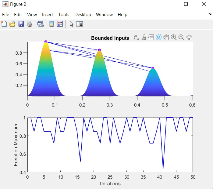
figure(2)                              % figure 2 for case 2
subplot(2,1,1)                         % specifying location for the graph in figure 2
hold on                                % holding the current graph
surfc(x,y,f)                           % plotting surface and contour using x, y and f
shading interp                         % interpolated shading
plot3(xopt2,yopt2,fval2,'color','b','marker','o','markersize',5,'markerfacecolor','m') % ploting lines in 3D space with the optimum values returned by ga in 3D space
title('Bounded Inputs')                % title for the graph
subplot(2,1,2)                         % specifying location for the graph in figure 2
plot(fval2,'color','b','linewidth',1)  % plotting a graph for fval2
xlabel('Iterations');                  % labelling x-axis
ylabel('Function Maximum');            % labelling y-axis

% Case 3: Statistical behaviour of GA by increasing the population size.

% modifying the default parameters using optimoptions
options = optimoptions('ga');
options = optimoptions(options,'PopulationSize',350); % changing the population size to 350
tic
for i = 1:num_cases                                                                      % initializing the for loop variable i
    [inputs3, fval3(i)] = ga(@stalagmite_ga,2,[],[],[],[],[0;0],[1;1],[],[],options);    % using this syntax to specify the population size through options and also specifying upper bound and lower bound
    xopt3(i) = inputs3(1);                                                               % assigning the returned optimum value of x by ga to xopt3
    yopt3(i) = inputs3(2);                                                               % assigning the returned optimum value of y by ga to yopt3
end

fval3 = -fval3;                       % this will convert the -ve values returned by ga as output to the positive value. (the stalagmite function (stalagmite_ga) was multiplied with -1)
Time_study3 = toc                     % stopping the timer for case 3 and assigning its value to the variable
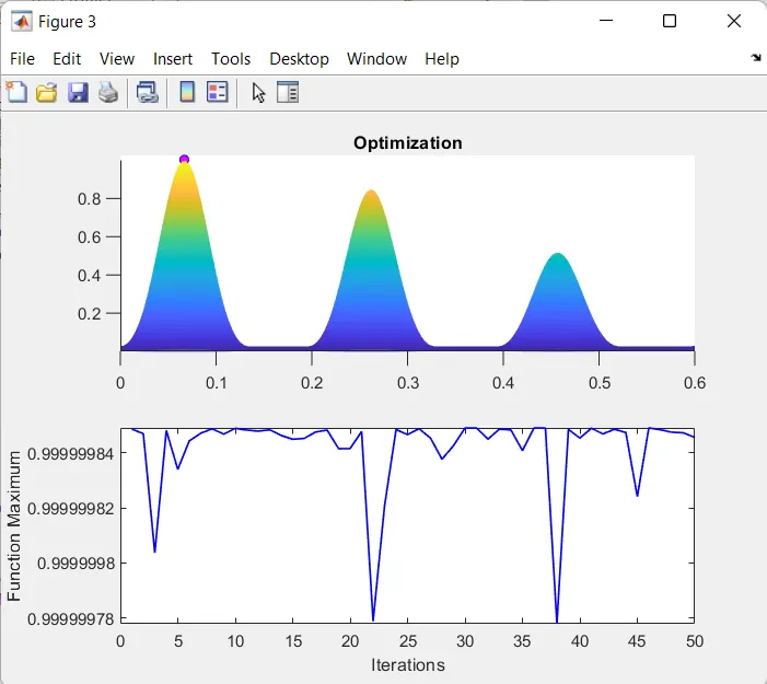
figure(3)                             % figure 3 for case 3
subplot(2,1,1)                        % specifying location for the graph in figure 2
hold on                               % holding the current graph
surfc(x,y,f)                          % plotting surface and contour using x, y and f
shading interp                        % interpolated shading
plot3(xopt3,yopt3,fval3,'color','b','marker','o','markersize',5,'markerfacecolor','m') % plotting lines in 3D space with the optimum values returned by ga in 3D space
title('Optimization')                 % title for the graph
subplot(2,1,2)                        % specifying location for the graph in figure 2
plot(fval3,'color','b','linewidth',1) % plotting a graph for fval3
xlabel('Iterations');                 % labelling x-axis
ylabel('Function Maximum');           % labelling y-axis