Week 2.1 - Air standard Cycle
MAIN SCRIPT
% Otto Cycle
clear
close all
clc

% Inputs
p1 = 101325;                            % pressure at state point 1
t1 = 500;                               % time at state point 1
t3 = 2300;                              % temperature at state point 3
gamma = 1.4;                            % specific heats ratio

% Engine geometric parameters (Inputs)
bore = 0.1;                             % bore dia
stroke = 0.1;                           % stroke length
con_rod = 0.15;                         % connecting rod length
cr = 12;                                % compression ratio (cr = v1/v2)


% Calculating the swept volume and the clearance volume

v_swept = (pi/4)*bore^2*stroke;         % swept volume
v_clearance = v_swept/(cr-1);           % clearance volume

v1 = v_swept + v_clearance;             % volume at state point 1
v2 = v_clearance;                       % volume at state point 2

% State varaibles at state point 2

% p2v2^gamma = p1v1^gamma  (isentropic compression process)
p2 = p1*(v1/v2)^gamma;                  % pressure at state point 2

% p1v1/t1 = p2v2/t2   (Ideal gas law)
t2 = p2*v2*t1/(p1*v1);                  % temperature at state point 2

% Volume trace for compression  (calling the function engine_kinematics)
V_compression = engine_kinematics(bore,stroke,con_rod,cr,180,0);

% Pressure trace for compression
% P_compression*V_compression^gamma = p1v1^gamma = constant  (isentropic process)
P_compression = (p1*v1^gamma)./(V_compression.^gamma);


% State variables at state point 3
% constant volume heat addition process
v3 = v2;                                % volume at state point 3

% p3v3/t3 = p2v2/t2   (Ideal gas law)
p3 = p2*t3/t2;                          % pressure at state point 3

% Volume trace for expansion   (calling the function engine_kinematics)
V_expansion = engine_kinematics(bore,stroke,con_rod,cr,0,180);

% Pressure trace for expansion
% P_expansion*V_expansion^gamma = p3v3^gamma = constant  (isentropic process)
P_expansion = (p3*v3^gamma)./(V_expansion.^gamma);

% State variables at state point 4
% constant volume heat rejection
v4 = v1;                                % volume at state point 4

% p3v3^gamma = p4v4^gamma (isentropic expansion process)
p4 = p3*(v3/v4)^gamma;                  % pressure at state point 4

% Thermal efficiency (otto cycle)
% efficiency_otto = 1 - 1/(cr^(gamma-1)) = 1 - t1/t2

eff_otto = 100*(1 - 1/(cr^(gamma-1)));

fprintf('The thermal efficiency of the engine for the Otto Cycle is %.2f percent.n',eff_otto)


% plotting volume and pressure points
figure(1)
hold on
plot(v1,p1,'*','color','r')
plot(v2,p2,'*','color','b')
plot(v3,p3,'*','color','g')
plot(v4,p4,'*','color','k')
xlabel('Volume')
ylabel('Pressure')
legend('(v1,p1)','(v2,p2)','(v3,p3)','(v4,p4)')

% plotting PV Diagram
figure(2)
hold on
plot(V_compression,P_compression)
plot([v2 v3],[p2 p3])
plot(V_expansion,P_expansion)
plot([v4 v1],[p4 p1])
xlabel('Volume')
ylabel('Pressure')
title('Otto Cycle - PV Diagram')
legend('isentropic compression','constant volume heat addition','isentropic expansion','constant volume heat rejection')
User defined function - engine_kinematics
function [V] = engine_kinematics(bore,stroke,con_rod,cr,start_crank,end_crank)

% function to determine the change in volume inside the combustion chamber
% with respect to crank postion given by crank angle (theta)

a=stroke/2;    % crank pin radius
R=con_rod/a;   % ratio of connecting rod length and crank pin radius

% Calculating swept volume and clearance volume
v_s=pi/4*bore^2*stroke;     % swept volume
v_c=v_s/(cr-1);             % clearance volume

theta = linspace(start_crank,end_crank,100);    % theta is the crank angle

% formula to determine change in volume inside the combustion chamber
%     V/v_c = 1 + (1/2)*(cr-1)*[R+1-cos(theta) - (R^2-sin^2(theta)^(1/2)]

term1 = 0.5*(cr-1);
term2 = R+1-cosd(theta);
term3 = (R^2 - sind(theta).^2).^0.5;

% Change in volume with respect to crank angle (theta)
V = (1+term1*(term2-term3)).*v_c;

end
The objective of this program is to:
1) Calculate unknown state variables (Pressure, Volume and Temperature) at all the state points for Otto cylce.
2) Calculate the thermal efficiency of the engine.
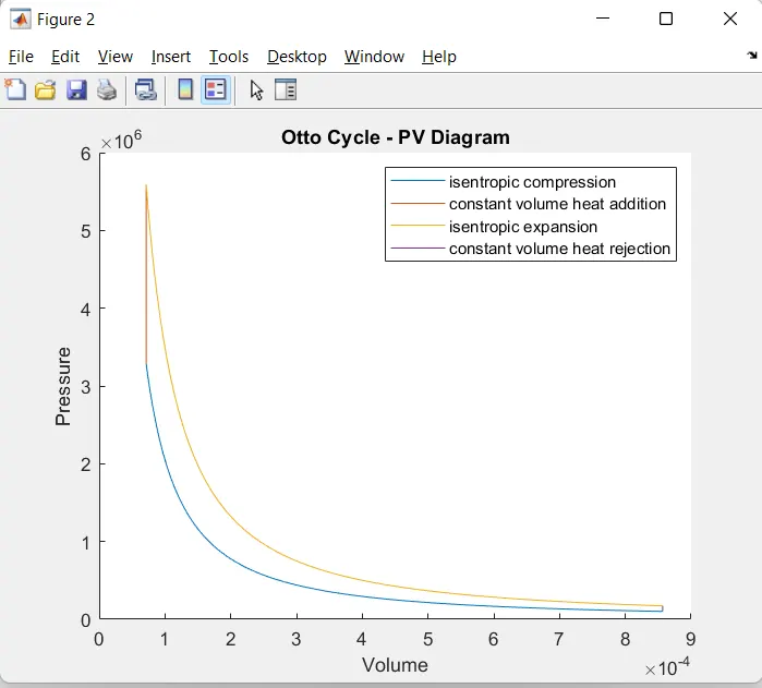
3) Plot a PV Diagram for the otto cycle.
Otto Cycle
State point 1 to 2 - Isentropic compression (p1v1^gamma = p2v2^gamma = constant)
State point 2 to 3 - Constant volume heat addition
State point 3 to 4 - Isentropic expansion (p3v3^gamma = p4v4^gamma = constant)
State point 4 to 1 - Constant volume heat rejection
Explanation of the User defined function (engine_kinematics)
I have created a function engine_kinematics which I'll be calling inside the main script. This function will determine the change in volume corresponding to the change in piston position. The piston position can be detemined by crank angle (theta).
The function will give one output argument (V) and require six input arguments (bore, stroke, con_rod, cr, start_crank, end_crank) while calling it.
function [V] = engine_kinematics(bore,stroke,con_rod,cr,start_crank,end_crank)
Inside the function I've initialized two variables a and R. a is the crank pin radius and R is the ratio of connecting rod length and crank pin radius.
a=stroke/2;
R=con_rod/a;
Then I've calculated swept volume and clearance volume inside the function and assigned them to variables v_s and v_c respectively.
v_s=pi/4*bore^2*stroke;
v_c=v_s/(cr-1);
Afterward I've initialized variable theta for the crank angle using funciton linspace which will give 100 data points from start crank angle (start_crank) to end crank angle (end_crank).
theta = linspace(start_crank,end_crank,100);
Then I've defined the formula that calculated the change in volume with respect to theta. The formula is
V/v_c = 1 + (1/2)*(cr-1)*[R+1-cos(theta) - (R^2-sin^2(theta)^(1/2)]
I've divided the formula into three terms and assigned three variables term1, term2 and term3.
term1 = 0.5*(cr-1);
term2 = R+1-cosd(theta);
term3 = (R^2 - sind(theta).^2).^0.5;
Finally I've put all the variables together to form an expression to calculate the volume change and have assigned it to variable V
V = (1+term1*(term2-term3)).*v_c;
Note: Since theta is an array (.*) and (.^) operators are used for mathematical operations.
end command - to close the function
The name of the function and .m file should be exactly same and it should be saved to the same directory where the main script is saved.
Explanation of the main script
Firstly I've assigned the values of known state variables, constants and engine parameters to the variables. These will be used as Inputs for the program.
pressure at state point 1 (p1), temperature at state point 1 (t1), temperature at state point 3 (t3), the specific heats ratio (gamma), stroke length (stroke), connecting rod length (con_rod) and compression ratio (cr)
First I have calculated swept volume and clearance volume using the mathematical expressions and assigned them to the variables v_swept and v_clearance.
v_swept = (pi/4)*bore^2*stroke;
v_clearance = v_swept/(cr-1);
Then using swept volume and clearance volume I've calculated volume at state point 1 and assigned it to v1 and calculated volume at state point 2 and assigned it to v2.
v1 = v_swept + v_clearance;
v2 = v_clearance
Next the calculation of state variables at state point 2.
From state point 1 to state point 2 is an isentropic compression process. So, p1v1^gamma = p2v2^gamma = constant. Using this expression I've calculated pressure at state point 2 and assigned it to variable p2.
p2 = p1*(v1/v2)^gamma;
Then by using Ideal Gas Law (p1v1/t1 = p2v2/t2 = constant) I've calculated temperature at state point 2 and assigned it to variable t2.
t2 = p2*v2*t1/(p1*v1);
Now to determine the change in volume inside the combustion chamber corresponding to the change in crank angle (theta) during compression process I've called the function engine_kinematics and put in the input arguments required and assigned it to variable named V_compression.
V_compression = engine_kinematics(bore,stroke,con_rod,cr,180,0);
In the above expression 180 is the start crank angle and 0 is the end crank angle meaning the piston is moving from bottom dead centre to top dead centre during compression process.
Then I've calculated the change in pressure during compression corresponding to the crank angle (theta) and assigned it to variable P_compression. Expression used here is
P_compression = (p1*v1^gamma)./(V_compression.^gamma)
Since V_compression and P_compression are arrays, therefore, operators (./) and (.^) are used for the maths operations.
Now the calculation of state variable at state point 3
Since the process from state point 2 to 3 is a constant volume process, the volume at point 3 will be equal to the volume at point 2. I've assined variable v3 for volume at point 3.
v3 = v2;
now pressure at point 3 is calculated by using ideal gas law (p3v3/t3 = p2v2/t2). t3 is known and initialized in the begining of the program. Value of pressure at point 3 is assigned to p3.
p3 = p2*t3/t2;
Now to calculate the volume change from state point 3 to 4 during expansion process I've again called the function engine_kinematics and assigned the output to variable V_expansion.
V_expansion = engine_kinematics(bore,stroke,con_rod,cr,0,180);
In the above expression the start crank angle is 0 and the end crank angle is 180. which means the piston is moving from Top dead centre to Bottom dead centre during expansion process.
After this I've calculated the change in pressure during expansion corresponding to the crank angle (theta) and assigned it to variable P_expansion. Expression used here is
P_expansion = (p1*v1^gamma)./(V_expansion.^gamma)
Calculating state variable at state point 4
Since the process from state point 4 to 1 is a constant volume process, the volume at point 4 will be equal to the volume at point 1. I've assigned variable v4 for volume at point 4.
v4 = v1;
From state point 3 to state point 4 is an isentropic expansion process. So, p3v3^gamma = p4v4^gamma = constant. Using this expression I've calculated pressure at state point 4 and assigned it to variable p4.
p4 = p3*(v3/v4)^gamma
Now I've calculated the thermal efficiency using the formula
eff_otto = 1 - 1/(cr^(gamma-1));
eff_otto is the variable assigned to the value of efficiency.
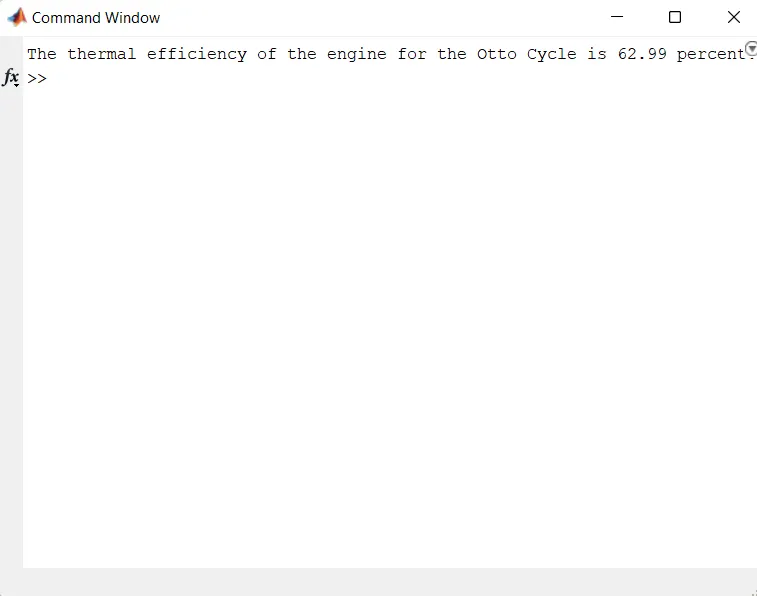
I've printed the output for the thermal efficiency using fprintf command.
fprintf('The efficiency of the otto cycle is %.2fn',eff_otto)
Now for plotting I've used two figures.
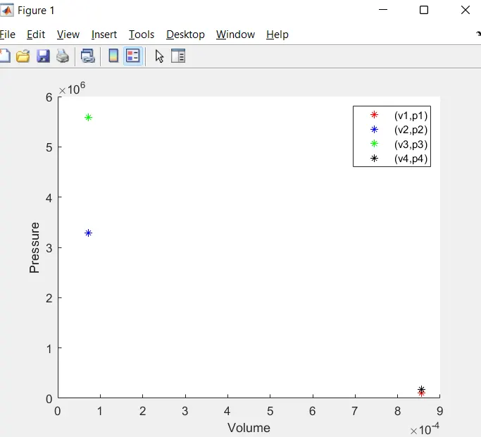
In first figure I've plotted the values of volume and pressure for all the state condition. (v1,p1), (v2,p2), (v3,p3), (v4,p4). I've labelled the the x and y axes using command xlabel and ylabel. legend command is used to create legend for the graph.
comand figure(1) is used to plot in first figure.
command hold on is used to plot all plots in figure 1.
plot(v1,p1,'*','color','r') - plotting v1 and p1 with * marker and red color
plot(v2,p2,'*','color','b') - plotting v2 and p2 with * marker and blue color
plot(v3,p3,'*','color','g') - plotting v3 and p3 with * marker and green color
plot(v4,p4,'*','color','k') - plotting v4 and p4 with * marker and black color
xlabel('Volume') - label for x-axis - 'Volume'
ylabel('Pressure') - label for y-axis - 'Pressure'
legend('(v1,p1)','(v2,p2)','(v3,p3)','(v4,p4)') - legend for the plot
In the second figure I've plotted the PV Diagram.
Again command figure(2) is used to create second figure.
hold on is used to plot all the plots in figure(2).
plot(V_compression,P_compression) - plotting isentropic compression process from state point 1 to point 2
plot([v2 v3],[p2 p3]) - plotting constant volume heat addition process from state point 2 to point 3
plot(V_expansion,P_expansion) - plotting isentropic expansion process from state point 3 to point 4
plot([v4 v1],[p4 p1]) - plotting constant volume heat rejection process from state point 4 to point 1
xlabel('Volume') - label for x-axis 'Volume'
ylabel('Pressure') - label for y-axis 'Pressure'
title('Otto Cycle - PV Diagram') - Creating Title for the plot
legend('isentropic compression','constant volume heat - addition','isentropic expansion','constant volume heat rejection') - legends for PV diagram. It will indicate all the colors used for plotting all the four processes.