Week 4.1 - Genetic Algorithm

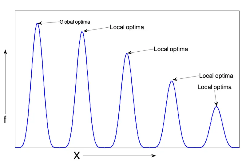
AIM: - To optimize the stalagmite function and find the global maxima of the function.

THEORY: - Genetic Algorithm (GA) is a search-based optimization technique based on the principles of Genetics and Natural Selection. It is frequently used to find optimal or near-optimal solutions to difficult problems which otherwise would take a lifetime to solve. It is frequently used to solve optimization problems, in research, and in machine learning.

GAs were developed by John Holland and his students and colleagues at the University of Michigan, most notably David E. Goldberg and has since been tried on various optimization problems with a high degree of success.

Below the following chart shows how the genetic algorithm works to find the optimum solution.

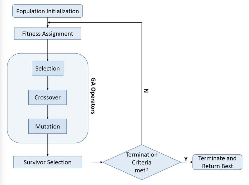
The format for writing genetic algorithm in matlab

x = ga(fun,nvars,A,b,Aeq,beq,lb,ub,nonlcon,intcon,options)

where: -

x is the local minima point.

Fun is the function to be called.

nvars indicates the no of variables used.

A and b are used to indicate any kind inequalities that exist in the function.

Lb = lower bound

Ub = upper bound

Nonlcon gives a two vectors representing inequalities and equalities.

Options is used to perform additional operations like increasing population size is done with “optioptions’’.

STALAGMITE FUNCTION:

A stalagmite is an upward-growing mound of mineral deposits that have precipitated from water dripping onto the floor of a cave. The fiqures we gets is in the shape of stalagmite so we use this name here. These formulas are represented in the below code.

`f(x,y)= f_1,_xf_2,_xf_1,_yf_2,_y`

`f_1._x=[sin(5.1pix+0.5)]^6`

`f_1._y=[sin(5.1piy+0.5)]^6`

`f_2,_x=exp[-4ln(2)(x-0.0667)^6 /(0.64)]`

`f_2,_y=exp[-4ln(2)(y-0.0667)^6 /(0.64)]`

PROGRAM: Defining Function Code

function [f] = stalagmite(input_vector)
x = input_vector(1);
y = input_vector(2);

a = [sin(5.1*pi*x+0.5)]^6;
b = [sin(5.1*pi*y+0.5)]^6;
c = exp(-4*log(2)*((x-0.0667).^2)/0.64);
d = exp(-4*log(2)*((y-0.0667).^2)/0.64);
f = (a*b*c*d);
end

Optimization code: -

close all
clear all
clc

% creating seaech space
x = linspace(0,0.6,150);
y = linspace(0,0.6,150);

%creating a 2-Dimensional mesh
[xx,yy] = meshgrid(x,y);

%evaluating the stalagamite function
for i = 1:length(xx)
    for j = 1:length(yy)
        input_vector(1) = xx(i,j);
        input_vector(2) = yy(i,j);
        f(i,j) = stalagmite(input_vector);
    end
end

surfc(xx,yy,f)
xlabel('x value')
ylabel('y value')

shading interp

CODE FOR ALL THREE STUDIES: -

close all
clear 
clc

x = linspace(0,0.6,150);
y = linspace(0,0.6,150);
num_cases = 60;

%creating a 2-Dimensional mesh
[xx,yy] = meshgrid(x,y);

%evaluating the stalagamite function
for i = 1:length(xx)
    for j = 1:length(yy)
        input_vector(1) = xx(i,j);
        input_vector(2) = yy(i,j);
        f(i,j) = stalagmite(input_vector);
    end
end


tic
% study 1-Statistical behavior
for i = 1:num_cases
    [inputs,fopt(i)] = ga(@stalagmite,2);
    xopt(i) = inputs(1);
    yopt(i) = inputs(2);
    
end

fopt = -fopt;

figure(1)
study1_time = toc;
subplot(2,1,1)
hold on
surfc(x, y, f)
shading interp
plot3(xopt,yopt,fopt,'marker','o','markersize',5,'markerfacecolor','r')
title('unbounded inputs')
subplot(2,1,2)
plot(fopt)
xlabel('iterations')
ylabel('function maxima')


tic
% study 2-Statistical behavior with upper bound and lower bound
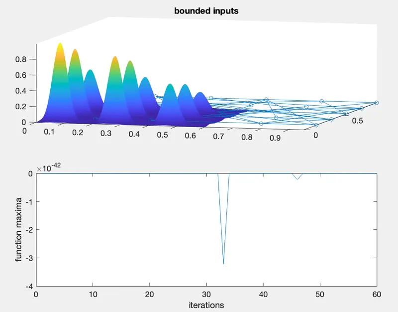
for i = 1:num_cases
    [inputs, fopt(i)] = ga(@stalagmite,2,[],[],[],[],[0;0],[1;1]);
    xopt(i) = inputs(1);
    yopt(i) = inputs(2);
end
fopt = -fopt;

study2_time = toc;
figure(2)
subplot(2,1,1)
hold on
surfc(x,y,f)
shading interp
plot3(xopt,yopt,fopt,'Marker','o','MarkerSize',5)
title('bounded inputs')
subplot(2,1,2)
plot(fopt)
xlabel('iterations')
ylabel('function maxima')

% study 3 increasing GA iterations
options = optimoptions('ga');
options = optimoptions(options,'PopulationSize',170);

tic
for i = 1:num_cases
    [inputs, fopt(i)] = ga(@stalagmite,2,[],[],[],[],[0;0],[1;1],[],[],options);
    xopt(i) = inputs(1);
    yopt(i) = inputs(2);
end
fopt = -fopt;

studytime3 = toc;
figure(3)
subplot(2,1,1)
hold on
surfc(x,y,f)
shading interp
plot3(xopt,yopt,fopt,'marker','o','markersize',5)
title('optimization')
subplot(2,1,2)
plot(fopt)
xlabel('iterations')
ylabel('function maximum')

Explanaton: -

• Program start with close all, clear all, and clc to close all previous plot, table,and commands
• X = linspace and y = linspace are input arrays of x and y.
• Num cases is used to run the genetic algorithm no. of times
• Meshgrid is used to store the value in 2d array
• Now we are calling ga value.
• The study 1- with unbounded inputs, a function loop applied running with num cases and ga value. The study time 1^st plot is calculated, also subplot is applied here.
• The study 2- with bounded inputs includes calling our predefined function loop as in first study. But here ga syntax defined along with range of inputs.
• The study 3- with in option followed with functional loop. In this study we increase the number of population size.

Figure 1.

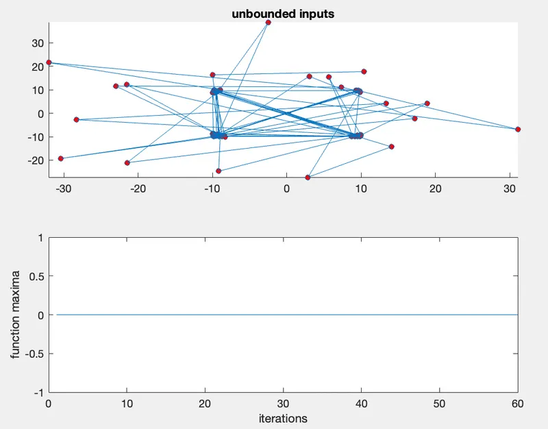
Figure 2.

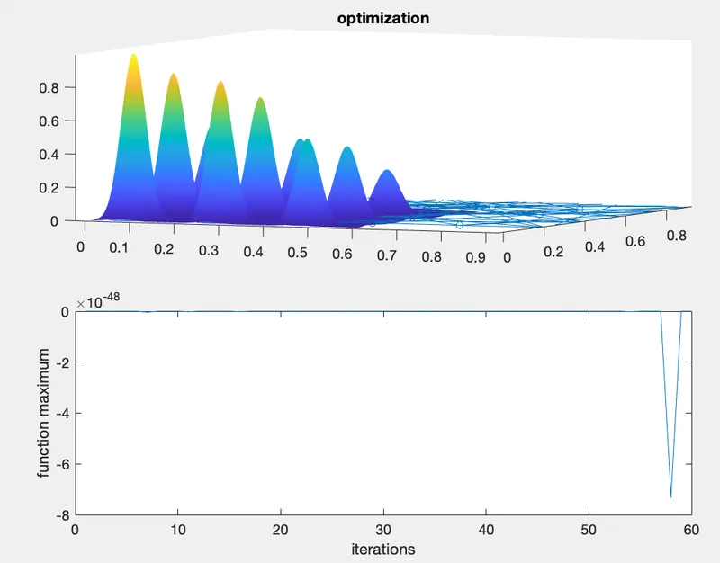
Figure 3.

errors.

there is a small problem with software the "Global optimization tool" doesnt support with trail version.

solution: i tried a lot to get out of it, finally taken help from 'request one to one'

in one to one session some errors had been corrected and the program got corrected but when i run same code in my trail version it show different result.