Week 4.1 - Genetic Algorithm

Aim:-

• Write a code in MATLAB to optimize the stalagmite function and find the global maxima of the function

• Explain the concept of genetic algorithms

• and also explain the syntax for ga in MATLAB.

• Plot graphs for all 3 studies and for F maximum vs no. of iterations.

• Significance of running multiple iterations and cases.

Concept of genetic algorithms:-

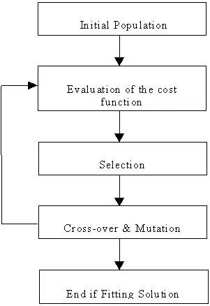
ga is an inbuilt solver in Matlab which is developed on the basis of the Theory of evolution.

The main idea of genetic algorithms is to evolve the best possible solution from random elements.

A genetic algorithm is working with a set of components, called chromosomes, which are initially randomly chosen in the parameter space. We call this set the population.

Syntax for ga in MATLAB:-

x = ga(fun,nvars,A,b,Aeq,beq,lb,ub,nonlcon,options)

[x,fval,exitflag,output,population,scores] = ga(___)

X- Solution, returned as a real vector. x is the best point that ga located during its iterations. If we have multiple variables then instead of x we can use inputs.

fun- This is an objective function of function handle for which the optimum solution we want to find.

nvars- no of variables in the objective function.

A and b- It is a Linear inequality constraint, which is specified as a real matrix.

A*x <= b,

For example, to specify

x + 2y ≤ 10

3x + 4y ≤ 20

5x + 6y ≤ 30,

A = [1,2;3,4;5,6];

b = [10;20;30];

Aeq and beq- It is a Linear inequality constraint, which is specified as a real vector.

Aeq*x = beq,

For example, to specify

x1 + 2x2 + 3x3 = 10

2x1 + 4x2 + x3 = 20,

Aeq = [1,2,3;2,4,1];

beq = [10;20];

lb and ub- It is a boundary condition for the variables.

lb- lower bounds

ub- upper bounds

If there are x and y are two variables and lb=[0,0], ub=[1,1]

Then the lower bound for x = 0 and y = 0, respectively added in lb arry.

the upper bound for x = 1 and y = 1, respectively added in ub arry.

nonlcon-

It is a nonlinear constraint, which is specified as a function handle or function name.

For example,

x = ga(@myfun,4,A,b,Aeq,beq,lb,ub,@mycon)

where mycon is a MATLAB® function such as

function [c,ceq] = mycon(x)

c = ... % Compute nonlinear inequalities at x.

ceq = ... % Compute nonlinear equalities at x.

options- It is a selection of options that will define initial population size, population size, plot function etc.

For example,

options = optimoptions(‘ga’, 'populationsize', 200)

200- is size of population

fval- This is Objective function value at the solution. Generally, fval = fun(x).

exitflag- Reason that ga stopped.

output- Information about the optimization process

population- Final population, returned as a PopulationSize-by-nvars matrix.

Significance of running multiple iterations and cases:-

1. Unbounded Statical behavior- it means that there is no lower bound and upper bound.
2. Bounded Statical behavior- Here we provide lower and upper limits in such a way that the search space is reduced with upper and lower boundaries.
3. 'bounded with population' Statical behavior- In this method, by using ‘optimoption’ command we bound the population size.

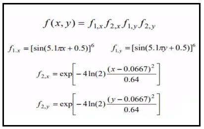
stalagmite function-

Code:-

stalagmite function-

function [f] = stalagmite(input_vector)
x = input_vector(1);
y = input_vector(2);
f1 = (sin(5.1*pi*x+0.5))^6;
f2 = (sin(5.1*pi*y+0.5))^6;
f3 = exp(-4*log(2)*(x-0.0667)^2/0.64);
f4 = exp(-4*log(2)*(y-0.0667)^2/0.64);
f = -(f1*f2*f3*f4); % -ve added, Because ga only minimize a function
end

Code for all 3 cases to optimize -

clear all
close all
clc
 
 % Defining our search space
 x = linspace(0,0.6,150);
 y = linspace(0,0.6,150);
 number_cases = 50; % Number of iteration to run ga is 50
 % Creating a 2D mesh
 [xx, yy] =  meshgrid(x,y);
 
 % Evaluating the Stalagmite function
 for i = 1:length(xx)
    for j = 1:length(yy)
     input_vector(1) = xx(i,j);
     input_vector(2) = yy(i,j);
     f(i,j) = stalagmite(input_vector);
    end
 end
 
 % Study case - 1 Unbounded Statical behaviour of Genetic Algorithm
 tic
 for k = 1:number_cases
 [inputs, fopt(k)] = ga(@stalagmite, 2);
 xopt(k) = inputs(1);
 yopt(k) = inputs(2);
 end
 study3_time = toc;
 
 %plotting
 figure(1)
 subplot(2,1,1)
 hold on
 surfc(x,y,f)
 hold on
 shading interp
 plot3(xopt, yopt, fopt, 'marker', 'o', 'markersize', 5, 'markerfacecolor', 'r')
 title('unbounded_input')
 subplot(2,1,2)
 plot(fopt)
 xlabel('Iteration')
 ylabel('Function Maximum Value')
 
 % Study case - 2 bounded Statical behaviour of Genetic Algorithm
 % lower boundary for x and y lb = [0,0]
 % upper boundary for x and y ub = [1,1]
  tic
 for k = 1:number_cases
 [inputs, fopt(k)] = ga(@stalagmite, 2, [], [], [], [], [0,0],[1,1]);
 xopt(k) = inputs(1);
 yopt(k) = inputs(2);
 end
 study2_time = toc;
 
 %plotting
 figure(2)
 subplot(2,1,1)
 hold on
 surfc(x,y,f)
 hold on
 shading interp
 plot3(xopt, yopt, fopt, 'marker', 'o', 'markersize', 5, 'markerfacecolor', 'r')
 title('unbounded_input')
 subplot(2,1,2)
 plot(-fopt)
 xlabel('Iteration')
 ylabel('Function Maximum Value')
 
  % Study case - 3 'bounded with population' Statical behaviour of Genetic Algorithm
  options = optimoptions('ga')
  options = optimoptions(options, 'populationsize', 200)
  tic
 for k = 1:number_cases
 [inputs, fopt(k)] = ga(@stalagmite, 2, [], [], [], [], [0,0],[1,1], [], [], options);
 xopt(k) = inputs(1);
 yopt(k) = inputs(2);
 end
 study1_time = toc;
 
 %plotting
 figure(3)
 subplot(2,1,1)
 hold on
 surfc(x,y,f)
 hold on
 shading interp
 plot3(xopt, yopt, -fopt, 'marker', 'o', 'markersize', 5, 'markerfacecolor', 'r')
 title('unbounded_input')
 subplot(2,1,2)
 plot(-fopt)
 xlabel('Iteration')
 ylabel('Function Maximum Value')

Output:-

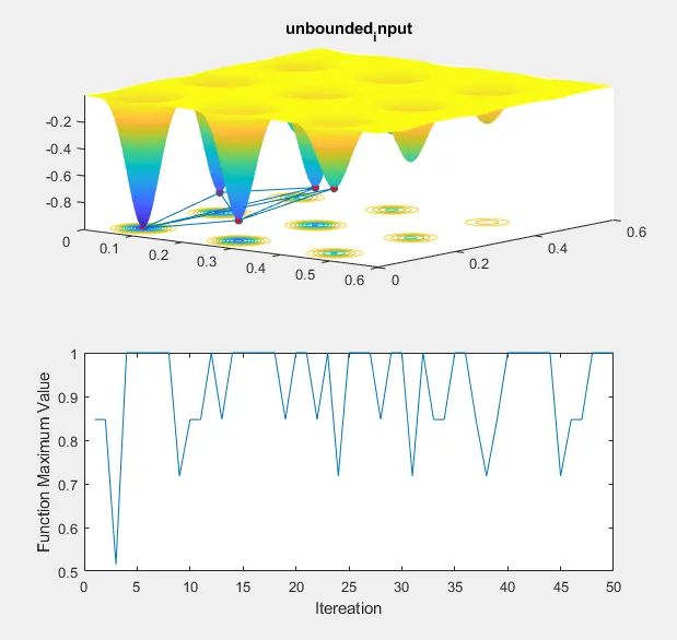
For Study case - 1 Unbounded Statical behavior of Genetic Algorithm

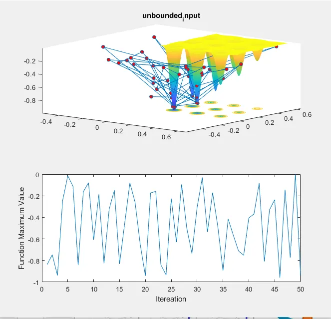
For Study case - 2 bounded Statical behavior of Genetic Algorithm

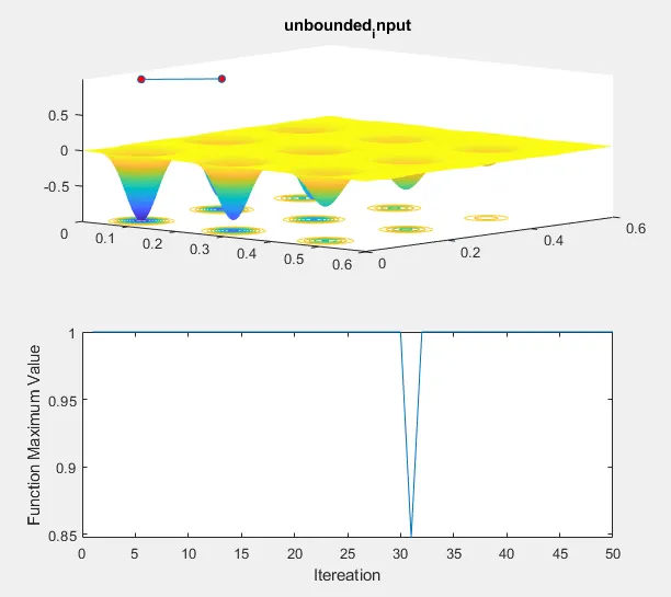
For Study case - 3 'bounded with population' Statical behavior of Genetic Algorithm

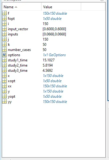
Workspace