Project 2 - Rankine cycle Simulator

Aim:-

1. Create a Rankine Cycle Simulator using OCTAVE/MATLAB.
2. Your code should calculate the state points of the Rankine Cycle (any type of your choice) based on user inputs.
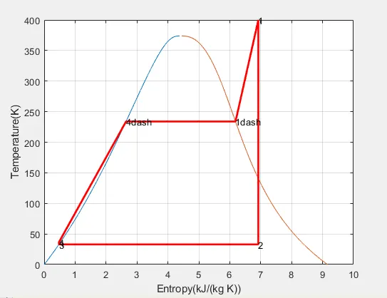
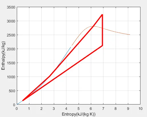
3. Then, plot the corresponding T-s and h-s plots for the given set of inputs. Title and axes labels are a must, while legends could be used if necessary.
4. Attach a report explaining the working of a Rankine cycle simulator and also the research done by you.
5. Calculate the followings,

• Net work output
• Back work ratio

Required Inputs:

Turbine Inlet temperature(t2) = 400° C

Turbine Inlet Pressure(p2) = 30 bars

Turbine Outlet Pressure(p3) = 0.05 bars = Condenser Inlet Pressure(p3)

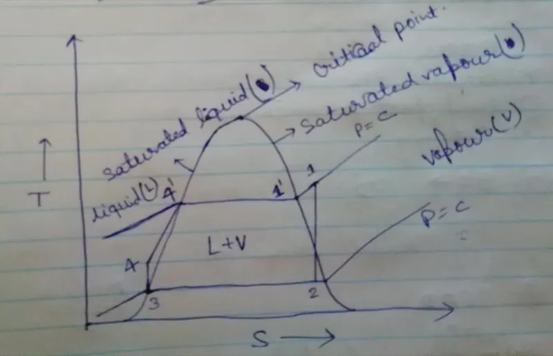
Working of a rankine cycle:-

Code:-

close all
clear all
clc

disp('Rankein Cycle Simulator')
disp('Process 1-2 Isentropic Expansion In Turbine')
disp('Process 2-3 Constant Pressure Heat Rejection by condenser')
disp('Process 3-4 Isentropic Compression in the pump')
disp('Process 4-1 Constant Pressure Heat Addition By Boiler')
% Input
% Turbine Inlet temperature(t1) = 400° C
% Turbine Inlet Pressure(p1) = 30 bars
% Turbine Outlet Pressure(p2) = 0.05 bars = Condenser Inlet Pressure(p2)
t1 = input('Enter Turbine Inlet temperature(t1)');
p1 = input('Turbine Inlet Pressure(p1)');
p2 = input('Turbine Outlet Pressure(p1)=Condenser Inlet Pressure(p2)');
% State 1
t1 = t1;
tv_sat = XSteam('Tsat_p',p1);
% as we can see t1>tsat; it means t1 is superheated steam
if t1>tv_sat
    h1 = XSteam('h_pt', p1,t1);
    s1 = XSteam('s_pt', p1,t1);
    else 
    t1 = tv_sat;
    h1 = XSteam('hV_p', p1);
    s1 = XSteam('sV_p', p1);
end    
% Calculation for State 2
% for isentropic (reversible adiabatic) process; s = constant
s2 = s1;
% s2 = s_f + x*s_fg
% x = dryness friction
s_f = XSteam('sL_p',p2);
s_g = XSteam('sV_p',p2);
s_fg = (s_g - s_f);
x = (s2-s_f)/s_fg;
% h2 = hf + x*h_fg
h_f = XSteam('hL_p',p2);
h_g = XSteam('hV_p',p2);
h_fg = (h_g - h_f);
h2 = h_f + x*h_fg;
t2 = XSteam('T_ps',p2,s2);

% Calculation for State 3
% For Constant Pressure p2 = p3;
% as we can see in T-S digram, Temperature is also constant
t3 = t2;
p3 = p2;
h3 = h_f;
s3 = XSteam('sL_p',p3);
v3 = XSteam('vL_p',p3);

% Calculation for state 4
% for isentropic compression(3-4)
s4 = s3;
p4 = p1; % for Constant Pressure (4-1)
% water is imcopmressable (v4 = v3)
v4 = v3;
% work done by pump = h4-h3
% v3(p4-p3) = h4-h3
h4 = h3 + v3*(p4-p3);
Cp = XSteam('cp_ps',p4,s4);
Cv = XSteam('cv_ps',p4,s4);
c = Cp/Cv;
t4 = t3*((p4/p3)^(c-1)/c);

% state 4_dash 
% p4 = p4_dash = p1_dash = p1;
p4_dash = p4;
t4_dash = tv_sat;
h4_dash = XSteam('hL_p',p4);
s4_dash = XSteam('sL_p',p4);
% state 1_dash
p1_dash = p1;
t1_dash = tv_sat;
h1_dash = XSteam('hV_p',p1);
s1_dash = XSteam('sV_p',p1);
% to find the curve of saturaed liquid and Vapour
T_critical = 374;
a = linspace(0,T_critical,5000);
for i = 1:length(a)
    sL(i)=XSteam('sL_T',a(i));
    sV(i)=XSteam('sV_T',a(i));
    hL(i)=XSteam('hL_T',a(i));
    hV(i)=XSteam('hV_T',a(i));
end
figure(1)
plot(sL,a)
hold on
plot(sV,a)

s = [s1,s2,s3,s4,s4_dash,s1_dash,s1];
t = [t1,t2,t3,t4,t4_dash,t1_dash,t1];
plot(s,t, 'linewidth',2,'color','r')
grid on
xlabel('Entropy(kJ/(kg K))')
ylabel('Temperature(K)')
text(s1,t1,'1')
text(s2,t2,'2')
text(s3,t3,'3')
text(s4,t4,'4')
text(s4_dash,t4_dash,'4dash')
text(s1_dash,t1_dash,'1dash')

figure(2)
plot(sL,hL)
hold on
plot(sV,hV)
h = [h1,h2,h3,h4,h4_dash,h1_dash,h1];
plot(s,h,'linewidth',3,'color','r')
grid on
xlabel('Entropy(kJ/(kg K))')
ylabel('Enthalpy(kJ/kg)')

% Work done by turbine
W_Turbine = h1-h2;
% Work done on the pump
W_pump = h4-h3;
% Net work Done by the cycle
W_net = W_Turbine - W_pump;
% Heat added on the boiler
Q_add = h1 - h4;
% Efficency of cycle
eff = W_net/Q_add;
% Back Work Ratio(BWR = Work done on condeser/work done by turbine)
BWR = (h2-h3)/(h1-h2);

disp('State 1')
fprintf('p1 = %f Bar, ', p1)
fprintf('t1 = %f Degree Celsius, ', t1)
fprintf('h1 = %f kJ/kg, ', h1)
fprintf('s1 = %f kJ/(kg K), ', s1)

fprintf('\n');
disp('State 2')
fprintf('p2 = %f Bar, ', p2)
fprintf('t2 = %f Degree Celsius, ', t2)
fprintf('h2 = %f kJ/kg, ', h2)
fprintf('s2 = %f kJ/(kg K), ', s2)

fprintf('\n');
disp('State 3')
fprintf('p3 = %f Bar, ', p3)
fprintf('t3 = %f Degree Celsius, ', t3)
fprintf('h3 = %f kJ/kg, ', h3)
fprintf('s3 = %f kJ/(kg K), ', s3)

fprintf('\n');
disp('State 4')
fprintf('p4 = %f Bar, ', p4)
fprintf('t4 = %f Degree Celsius, ', t4)
fprintf('h4 = %f kJ/kg, ', h4)
fprintf('s4 = %f kJ/(kg K), ', s4)

Output:-