Week 4.1 - Genetic Algorithm

Aim: To study the optimization of a function for finding Global Maxima with help of Genetic Algorithm

Objective:

1. To write a code for Global Maxima
2. To plot the outputs with labels
3. Theory about ga, stopping criteria, syntax for ga, significance of running multiple iterations and cases and results must be explained well

Genetic Algorithm:

The genetic algorithm is a method for solving both constrained and unconstrained optimization problems that is based on natural selection, the process that drives biological evolution. The genetic algorithm repeatedly modifies a population of individual solutions.

The genetic algorithm uses three main types of rules at each step to create the next generation from the current population:

• Selection rules select the individuals, called parents, that contribute to the population at the next generation.
• Crossover rules combine two parents to form children for the next generation.
• Mutation rules apply random changes to individual parents to form children.

Equations:

To find global maxima

`f=(f1.f2.f3.f4)`

To find global minima

`f=(f1.f2.f3.f4)`

Where

`f1=〖[sin⁡(5.1πx+0.5)]〗^6`

`f1=〖[sin⁡(5.1πy+0.5)]〗^6`

`f3=exp[-4log⁡(2)〖(x-0.0667)〗^2/0.64]`

`f4=exp[-4log⁡(2)(〖(y-0.0667)〗^2/0.64) ]`

Program Code to Plot

clear all
close all
clc

%defining our search space
x = linspace(0,0.6,150);
y = linspace(0,0.6,150);

% creating a 2Dimensional mesh
[xx,yy] = meshgrid(x,y);

%evaluating the stalagmite function
for i=1:length(xx)
    for j=1:length(yy)
        input_vector(1)=xx(i,j);
        input_vector(2)=yy(i,j);
        f(i,j)=stalagmite(input_vector);
    end 
end

surfc(xx,yy,f)
xlabel('x value');
ylabel('y value');

shading interp

[inputs, fval] = ga(@stalagmite, 2)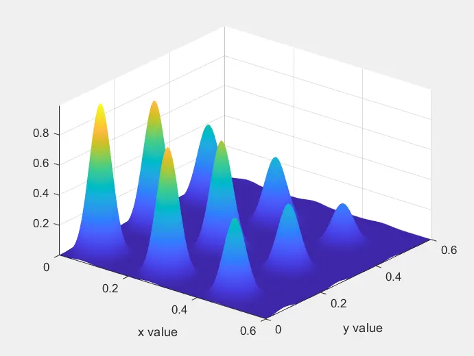

Function Code

function [f]=stalagmite(input_vector)

x= input_vector (1);
y= input_vector (2);
f1=(sin(5.1*pi*x+0.5))^6;
f2=(sin(5.1*pi*y+0.5))^6;
f3=exp(-4*log(2)*(x-0.0667)^2/0.64);
f4=exp(-4*log(2)*(y-0.0667)^2/0.64);

f=(f1*f2*f3*f4);
end

Study 1,2 and 3

clear all
close all
clc

%defining our search space
x = linspace(0,0.6,150);
y = linspace(0,0.6,150);
num_cases=50;
% creating a 2Dimensional mesh
[xx,yy] = meshgrid(x,y);

%evaluating the stalagmite function
for i=1:length(xx)
    for j=1:length(yy)
        input_vector(1)=xx(i,j);
        input_vector(2)=yy(i,j);
        f(i,j)=stalagmite(input_vector);
    end 
end

tic
%statistical behaviour- study 1
for i= 1:num_cases
    [inputs,fopt(i)]=ga(@stalagmite,2)
    xopt(i)=inputs(1)
    yopt(i)=inputs(2)
end

%plotting
figure(1)
subplot(2,1,1)
hold on
surfc(x,y,f)
hold on
shading interp
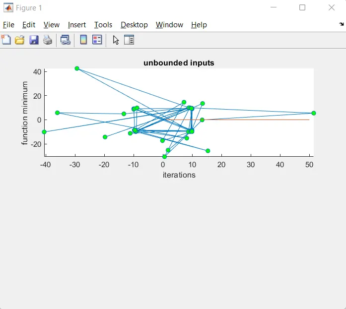
plot3(xopt,yopt,fopt,'marker','o','markersize',5,'markerfacecolor','g')
title('unbounded inputs')
subplot(2,1,1)
plot(fopt)
xlabel('iterations')
ylabel('function minimum')

tic
%study 2- statistical behaviour-upper and lower bounds

for i=1:num_cases
    [inputs,fpot(i)]=ga(@stalagmite,2,[],[],[],[],[0,0],[1,1]);
    xopt(i)= inputs(1)
    ypot(i)=inputs(2)
end

study2_time=toc;

%plotting
figure(2)
subplot(2,1,1)
hold on 
surfc(x,y,f)
hold on
shading interp
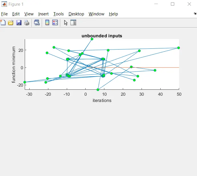
plot3(xopt,yopt,fopt,'marker','o','markersize',5,'markerfacecolor','g')
title('unbounded inputs')
subplot(2,1,1)
plot(fopt)
xlabel('iterations')
ylabel('function minimum')

%study 3
options = optimoptions ('ga');
options = optimoptions(options,'PopulationSize',250);
tic
for i=1:num_cases
    [inputs,fpot(i)]=ga(@stalagmite,2,[],[],[],[],[0,0],[1,1],[],[],options);
    xopt(i)= inputs(1)
    ypot(i)=inputs(2)
end

study3_time=toc;

%plotting
figure(2)
subplot(2,1,1)
hold on 
surfc(x,y,f)
hold on
shading interp
plot3(xopt,yopt,fopt,'marker','o','markersize',5,'markerfacecolor','g')
title('unbounded inputs')
subplot(2,1,1)
plot(fopt)
xlabel('iterations')
ylabel('function minimum')

Output