Week 2- 2R Robotic Arm Challenge

This is a detailed report of Kinematics of a Robotic Arm.

Robotics is an emerging field.

To solve this problem we need to understand the kinematics of linkages.

A robotic arm is a type of mechanical arm, usually programable, with similar functions to a human arm, the arm may be the sum total of the mechanism or may be part of a more complex robot. Robotic arms can be used for all manner of industrial production, processing and manufacturing roles - any task in which extremely precise, fast and repeatable movements are required.

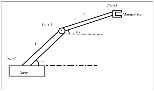
In the image shown above, the robotic arm consists of 4 components,

• The Base, which is clamped to the surface and all other links are joined through hinge joint.
• Link 1 (L1) making Ө 1 with horizontal.
• Link 2 (L2) making Ө 2 with horizontal.
• The device attached to the manipulator which interacts with its environment to perform tasks is called the end-effector.

Calculation

Step 1: To calculate position of link 1 by basic Trigonometry

Link 1 co-ordinates (0 0),(LcosӨ , Lsin Ө)

Step 2: To calculate position of link 2 by Trigonometry

As link 2 is a joint with link 1

X2= x1+L2cos Ө

Y2 = y1+L2sin Ө

INPUTS:

• For our program we have assumed the length of link 1 ,1m and link 2 ,0.5m
• In order to simulate the robotic arm it is necessary to vary Ө1 and Ө2 to obtain a desired animation and it cannot be possible if we manually enter the respective data everytime. So we have created a row vector from 0° - 90° with increment of 10 points between them using linspace command.

Program

close all
clear all
clc


%Inputs 
l1 = 1;
l2 = 0.5;

theta1 = linspace(0,90,10);
theta2 = linspace(0,90,10);

ct=1;   %Counter value will be 1
for i = 1:length(theta1)  
    THETA1= theta1(i);
    for j = 1:length(theta2)
        THETA2 = theta2(j);

% Co-ordinates of first arm start point
x0 = 0;
y0 = 0;

%Co-ordinates of end point first arm/ start point of 2nd arm
x1 = l1*cosd(THETA1);
y1 = l1*sind(THETA1);

%Co-ordinates of end point of 2nd arm
x2 = x1 + l2*cosd(THETA2);
y2 = y1 + l2*sind(THETA2);

%plotting
% Instead of using line command we use plot command to get all plots in one
% figure
plot([x0 x1],[y0 y1],[x1 x2],[y1 y2],'linewidth',3)
axis([-0.1 1.5 0 1.5])
pause(0.3)
M(ct)= getframe(gcf);
ct=ct+1;
    end 
end
% to create an animation of our plot we use the following commands
movie(M)
videofile = VideoWriter('forward_kinematic_with_for_loop.avi','uncompressed AVI');
open(videofile)
writeVideo(videofile,M)
close (videofile)
 

% Outputs

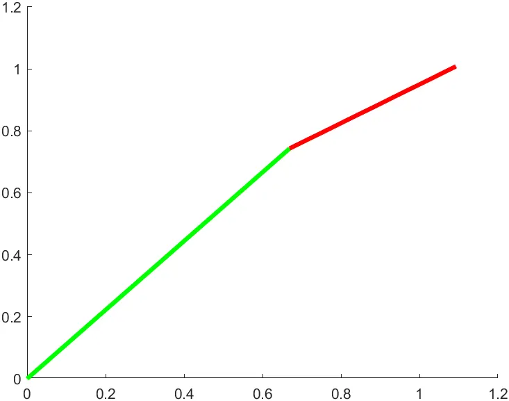
Animation Video Link

https://drive.google.com/file/d/1ujKlh8XXNn5z2TRPAt2gwDMwLqfRfs3i/view?usp=sharing

% Errors

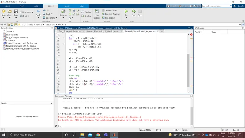
% Faced an error where one end for J was missing