Week 4.1 - Genetic Algorithm

THEORY:

Stalagmite:

• A stalagmite is an upward-growing mound of mineral deposits that have precipitated from water dripping onto the floor of a cave. Most stalagmites have rounded or flattened tips.

Equations:

The following equations have been used to reproduce stalagmite.

`a = sin ( ( 5.1 ⋅ π ⋅ x + 0.5 ) ) ^6`

`b = sin ( ( 5.1 ⋅ π ⋅ y + 0.5 ) ) ^6`

`c = e ^[− (( 4 ⋅ log ( 2 ) ) ⋅ ( x − 0.0667 ))^2/ 0.64]`

`d = e ^[− (( 4 ⋅ log ( 2 ) ) ⋅ ( y − 0.0667 ))^2/ 0.64]`

• [p,S,mu] = polyfit(x,y,n) also returns mu, which is a two-element vector with cantering and scaling values. mu(1) is mean(x), and mu(2) is std(x). Using these values, polyfit centres x at zero and scales it to have unit standard deviation,
  
  This centring and scaling transformation improves the numerical properties of both the polynomial and the fitting algorithm.

So by using [p,S,mu] = polyfit(x,y,n) we can improve the cubic fit further more.

Genetic algorithm:

The genetic algorithm is a method for solving both constrained and unconstrained optimization problems that is based on natural selection, the process that drives biological evolution. The genetic algorithm repeatedly modifies a population of individual solutions. At each step, the genetic algorithm selects individuals at random from the current population to be parents and uses them to produce the children for the next generation. Over successive generations, the population "evolves" toward an optimal solution. You can apply the genetic algorithm to solve a variety of optimization problems that are not well suited for standard optimization algorithms, including problems in which the objective function is discontinuous, nondifferentiable, stochastic, or highly nonlinear. The genetic algorithm can address problems of mixed integer programming, where some components are restricted to be integer-valued.

The genetic algorithm uses three main types of rules at each step to create the next generation from the current population:

• Selection rules select the individuals, called parents, that contribute to the population at the next generation.
• Crossover rules combine two parents to form children for the next generation.
• Mutation rules apply random changes to individual parents to form children.

The genetic algorithm differs from a classical, derivative-based, optimization algorithm in two main ways, as summarized in the following table.

Classical Algorithm	Genetic Algorithm
Generates a single point at each iteration. The sequence of points approaches an optimal solution.	Generates a population of points at each iteration. The best point in the population approaches an optimal solution.
Selects the next point in the sequence by a deterministic computation.	Selects the next population by computation which uses random number generators.

Outline of GA algorithm:

The following outline summarizes how the genetic algorithm works:

1. The algorithm begins by creating a random initial population.
2. The algorithm then creates a sequence of new populations. At each step, the algorithm uses the individuals in the current generation to create the next population. To create the new population, the algorithm performs the following steps:
1. Scores each member of the current population by computing its fitness value. These values are called the raw fitness scores.
2. Scales the raw fitness scores to convert them into a more usable range of values. These scaled values are called expectation values.
3. Selects members, called parents, based on their expectation.
4. Some of the individuals in the current population that have lower fitness are chosen as elite. These elite individuals are passed to the next population.
5. Produces children from the parents. Children are produced either by making random changes to a single parent—mutation—or by combining the vector entries of a pair of parents—crossover.
6. Replaces the current population with the children to form the next generation.
3. The algorithm stops when one of the stopping criteria is met.
4. The algorithm takes modified steps for linear and integer constraints.
5. The algorithm is further modified for nonlinear constraints.

A very detailed explanation is given in the below URL:
https://in.mathworks.com/help/gads/how-the-genetic-algorithm-works.html

Syntax for 'ga' algorithm:

• x = ga(fun,nvars)
  x = ga(fun,nvars) finds a local unconstrained minimum, x, to the objective function, fun. nvars is the dimension (number of design variables) of fun.
• x = ga(fitnessfcn,nvars,A,b,Aeq,beq,LB,UB)
  x = ga(fun,nvars,A,b,Aeq,beq,lb,ub) defines a set of lower and upper bounds on the design variables, x, so that a solution is found in the range lb ≤ x ≤ ub. (Set Aeq=[] and beq=[] if no linear equalities exist.)
• x = ga(fitnessfcn,nvars,A,b,[],[],LB,UB,nonlcon,IntCon,options)
  x = ga(fun,nvars,A,b,Aeq,beq,lb,ub,nonlcon,intcon) or x = ga(fun,nvars,A,b,Aeq,beq,lb,ub,nonlcon,intcon,options) requires that the variables listed in intcon take integer values.

Refer the below URL for meanings of each variable mentioned in the syntax:
https://in.mathworks.com/help/gads/ga.html#d123e44602

Function code:

Explanation:

• The function passed has one output variable named 'f' and the function is named 'stalagmite' and one input matrix with 2 elements is passed as argument.
• The equations for stalagmite are declared and the function is terminated with keyword 'end'.

function f = stalgamite(input_vector)

a=(5.1*pi*input_vector(1)+0.5);
b=(5.1*pi*input_vector(2)+0.5);
c=(-(4*log(2))*(input_vector(1)-0.0667)^2)/(0.64);
d=(-(4*log(2))*(input_vector(2)-0.0667)^2)/(0.64);

f_x1=(sin(a))^6;
f_y1=(sin(b))^6;
f_x2=exp(c);
f_y2=exp(d);

f=-f_x1*f_y1*f_x2*f_y2;

end

Code:

Explanation:

• The code starts with creating x and y coordinates for the stalagmite function to operate on.
• Mesh grid coordinates are generated for the coordinates
• The first two for loops run for the number of values of the mesh grid elements and the input vector elements are passed as the arguments to the function 'stalagmite'.
• The final for loop runs to execute the 'ga' solver and records the output values.
  The first 'ga' solver is for the unbounded case whereas the following cases are for bounded case (this restricts the grid to a particular value) and optimised case respectively.
  The change in syntax of the 'ga' solver must be noted.
• The arrays obtained are plotted as a surface plot and function minimum is plotted over the number of iterations.

clear all
close all
clc

x=linspace(0,0.6,150);
y=linspace(0,0.6,150);
num_cases=50;
[xx,yy]=meshgrid(x,y);
% f=meshgrid(x,y);

tic

%creating the stalgamite function
%for each value of x and y we are creating an input vector
%input vector is a row vector meaning it has 2 columns
for i = 1: length(xx)
    for j =1:length(yy)
        input_vector(1)=xx(i,j);
        input_vector(2)=yy(i,j);
        f(i,j)=stalgamite(input_vector);
    end
end
%study 1 - Statistical behaviour
for i=1:num_cases
    [inputs, fopt(i)]=ga(@stalgamite,2);
    xopt(i)=inputs(1);
    yopt(i)=inputs(2);
end
Study_time_1=toc

% surfc(x,y,f)
figure(1)
subplot(2,1,1)
surfc(x,y,-f)
shading interp
hold on
plot3(xopt,yopt,-fopt,'marker','o','markersize',5,'markerfacecolor','r')
title('Unbounded Inputs')
subplot(2,1,2)
plot(-fopt)
xlabel('Iterations')
ylabel('Function minimum')



% setting up of upper limit and lower limit for minima/maxima value
tic
for i=1:num_cases
    [inputs, fopt(i)]=ga(@stalgamite,2,[],[],[],[],[0;0],[0.6;0.6]);
    xopt(i)=inputs(1);
    yopt(i)=inputs(2);
end

Study_time_2=toc

figure(2)
subplot(2,1,1)
surfc(x,y,-f)
shading interp
hold on
plot3(xopt,yopt,-fopt,'marker','o','markersize',5,'markerfacecolor','r')
title('Bounded Inputs')
subplot(2,1,2)
plot(-fopt)
xlabel('Iterations')
ylabel('Function minimum')


%study 3 increasing GA iterations
options=optimoptions('ga');
options=optimoptions(options,'PopulationSize',300);

tic

for i=1:num_cases
    [inputs, fopt(i)]=ga(@stalgamite,2,[],[],[],[],[0;0],[0.6;0.6],[],[],options);
    xopt(i)=inputs(1);
    yopt(i)=inputs(2);
end

Study_time_3=toc

figure(3)
subplot(2,1,1)
surfc(x,y,-f)
shading interp
hold on
plot3(xopt,yopt,-fopt,'marker','o','markersize',5,'markerfacecolor','r')
title('Optimised Inputs')
subplot(2,1,2)
plot(-fopt)
xlabel('Iterations')
ylabel('Function minimum')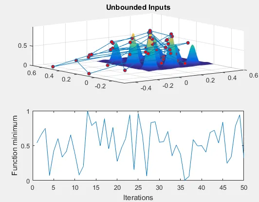

The minimum value of the function seems to lie all over the grid and doesn’t seem to make sense, while the function minimum plot looks highly irregular.

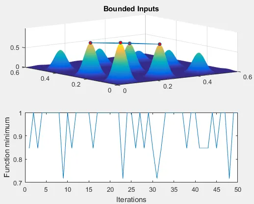
With the bounded case the irregularities in the plot minima estimation is reduced significantly, the function minima/maxima plot is less chaotic in comparison to the unbounded case.

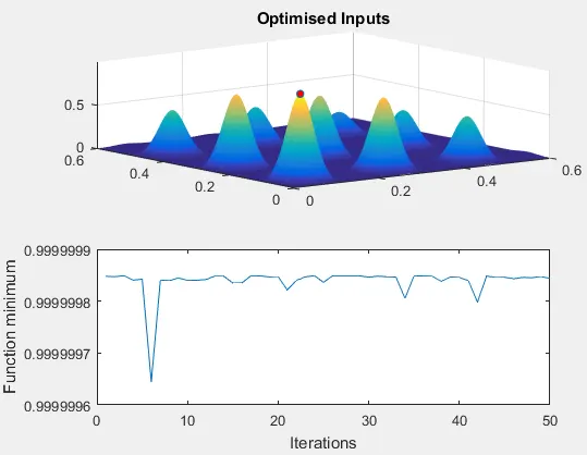
The optimised case which uses the 'ga' solver has correctly pointed out to the maxima/minima point for the stalagmite function. Also note the reduced variations in the function minimum.

Errors:

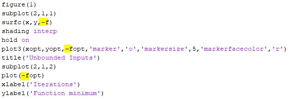
1. The negative sign in the final function statement is very important to obtain a meaningful plot.

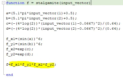
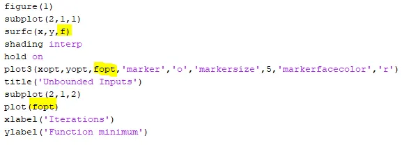
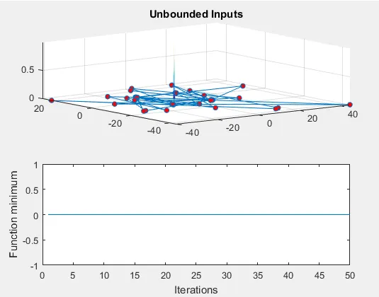
After adding the negative sign to the final equation in the function the plots obtained will be in an inverted fashion.

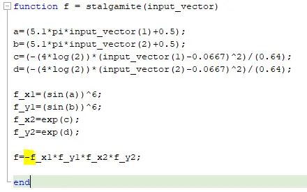
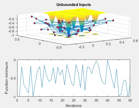
A negative sign must be added to the variables that involves the component of function call 'f' & 'fopt' to reverse the inverted stalagmite.

To avoid variation in the plot while running the code multiple times we must make sure to take note of the boundary value for case 2 and case 3.

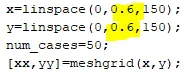
The value of x,y and boundary values mentioned in arguments in 'ga' solver must be same
If these values are not same then there will be significant variation in the plot.

Conclusion:

Having options and a population size will increase the accuracy of the prediction.

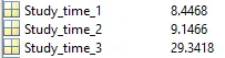
Note the change in study time for each case below, it can be clearly seen that for each additional constraint the computational power and time required to run the code is increasing.
The time required when using the 'ga' solver is more than thrice the time required to run the unbounded case.

References:

https://in.mathworks.com/help/gads/some-genetic-algorithm-terminology.html

https://in.mathworks.com/help/gads/what-is-the-genetic-algorithm.html

https://in.mathworks.com/help/gads/how-the-genetic-algorithm-works.html