Week 3 - Solving second order ODEs
Aim:
Objective is to write a program that solves the following ODE. This ODE represents the equation of motion of a simple pendulum with damping
In the above equation,
g = gravity in m/s2,
L = length of the pendulum in m,
m = mass of the ball in kg,
b=damping coefficient.
Objective:
Write a program in Python that will simulate the pendulum motion, just like the one shown in the start of this challenge.
use,
L=1 metre,
m=1 kg,
b=0.05,
g=9.81 m/s2
Simulate the motion between 0-20 sec, for angular displacement=0,angular velocity=3 rad/sec at time t=0.
Theory:
Idealised pendulum:
An idealised pendulum is a swinging rigid body free to rotate about a fixed horizontal axis, consisting of a massless string of length "l" which suspends a pendulum bob of mass "m" .In addition a damping factor "b" may act due to friction at the pivot or due to air resistance or both together could dampen motion .
When a pendulum is displaced sideways from its equilibrium position it is subjected to a restoring force due to gravity that will accelerate it back towards the equilibrium position .
When released the restoring force acting on the pendulum's mass causes it to oscillate about the equilibrium position ,swinging back and forth .
fig 1 : A pendulum with tangential and radial force components.
To find the arc length of the pendulum,
arc length ('s' in radians) =Radius ('r' in standard length) *theta (in radians)
`S=r*theta`
here, r=l
`(ds)/(dt)=l*(d(theta))/(dt)|`
`(d^2s)/(dt^2)=l*[(d^2(theta))/dt^2]`-------------(1)
Force, 'Fr' is countered by the tension due to the pivot and hence gets balanced.
so, 'Ft' is the only force we will have to focus on for further calculation.
The forces acting on the pendulum bob are ,
i) Damping factor(b)
ii) Air resistance
so,
`F=-[mg*sin(theta)]-[b*(d(theta))/(dt)]`-------------(2)
The negative sign in `-[mg*sin(theta)]`is present to denote the direction of motion in negative direction.
The negative sign `-[b*(d(theta))/(dt)]` is present to denote that the damping causes resistance to motion of pendulum bob and hence reduces the force.
By Newton's 2nd law,
`F=m*a`
`F=m*((d^2s)/(dt^2))`---------------------(3)
hence,
Equating (!) & (2),
`m*(d^2s)/(dt^2)=-[mg*sin(theta)]-[b*(d(theta))/dt]`--------------(4)
Substitute (1) & (2),
`m*l*[(d^2(theta))/(dt^2)]=-[mg*sin(theta)]-[b*(d(theta))/dt]`
`(d^2(theta))/(dt^2)=-[(g/l)*sin(theta)]-[{b/(m*l)}*(d(theta))/dt]`
Code:
Explanation:
- The code was written in python using the IDE Sublime text editor 3.
- Along with the regular libraries like nump, matplotlib.pyplot, math an additional new library that is imported here is the scipy from which we import scipy.integrate and specifically odeint.
- The function is passed with the name 'model' with input arguments 'theta, t, b, g, l, m.
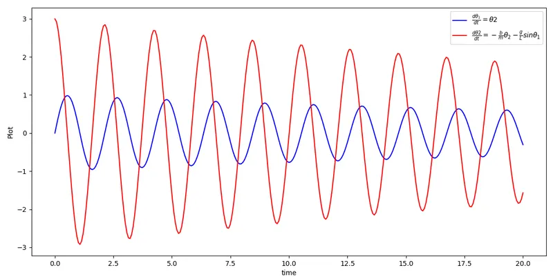
Here the first theta1 is the angular velocity, theta2 is the angular acceleration.
We initialise the angular velocity with theta2, and the angular acceleration is initialised by transposing the other terms to the RHS (`(d^2(theta))/(dt^2)=-[(g/l)*sin(theta)]-[{b/(m*l)}*(d(theta))/dt]`) - Then group the angular velocity and angular acceleration into a single matrix.
- The g is the gravity in m/s2, L is the length of the pendulum in m, m is the mass of the ball in kg, b is the damping coefficient.
- The initial condition for the pendulum bob is the angular velocity = 0, acceleration is 3rad/sec.
- The time points are set to 0 to 20 seconds with 300 time points in between the interval.
- The function is called and the arguments are passed within the odeint inbuilt function, it is a command that we use to integrate a function to linearise the equation in PDE.
- The time vs angular velocity & angular acceleration has been plotted on the same figure window to compare them both.
- The loop counter is introduced and the for loop is used to generate images of the change in pendulum bob at each time interval.
- The images are then uploaded to a free website that creates a video from by stitching the images together.
import numpy as np
from scipy.integrate import odeint
import matplotlib.pyplot as plt
import math

# function that returns dz/dt
def model(theta, t, b, g , l, m):
	theta1 = theta[0]
	theta2 = theta[1]
	dtheta1_dt = theta2
	dtheta2_dt = -(b/m)*theta2 - (g/l)*math.sin(theta1)
	dtheta_dt = [dtheta1_dt, dtheta2_dt]
	return dtheta_dt

b = 0.05
g = 9.81
l = 1
m = 1

# initial condition
theta_0 = [0, 3]

# time points
t = np.linspace(0, 20, 300)

# solve ODE
theta = odeint(model, theta_0, t, args = (b, g, l , m))

# plot results
plt.plot(t, theta[:, 0], 'b-', label = r'$\frac{d\theta_1}{dt} = \theta2$', color = 'blue')
plt.plot(t, theta[:, 1], 'b-', label = r'$\frac{d\theta2}{dt} = -\frac{b}{m}\theta_2-\frac{g}{L}sin\theta_1$', color = 'red')
plt.ylabel('Plot')
plt.xlabel('time')
plt.legend(loc = 'best')
plt.show()

print(theta[:, 0])
print(theta[:, 1])

ct = 1

for i in range(0, len(t)):

	x0 = 0
	y0 = 0

	# link one link two connector
	x1 = l*math.sin(theta[:, 0][i])
	y1 = -l*math.cos(theta[:, 0][i])

	filename = str(ct) + '.png'
	ct = ct+1

	# to animate plot
	# to plot the plot in a new figure window
	plt.figure()
	plt.plot([x0, x1], [y0, y1])
	plt.plot(x1, y1, 'o', markersize = 10)
	plt.xlim(-1.5, 1.5)
	plt.ylim(-1.5, 1.5)
	# plots one graph and saves figure in the folder same as the code
	plt.savefig(filename)
Code:
Animation:
From: https://ezgif.com/maker
Error code:
import numpy as np
from scipy.integrate import odeint
import matplotlib.pyplot as plt
import math

# function that returns dz/dt
def model(theta, t, b, g , l, m):
	theta1 = theta[0]
	theta2 = theta[1]
	dtheta1_dt = theta2
	dtheta2_dt = -(b/m)*theta2 - (g/l)*math.sin(theta1)
	dtheta_dt = [dtheta1_dt, dtheta2_dt]
	return dtheta_dt

b = 0.02
g = 9.81
l = 1
m = 0.1

# initial condition
theta_0 = [math.pi/4, 0]     # initial position of the pendulum bob

# time points
t = np.linspace(0, 10, 150)

# solve ODE
theta = odeint(model, theta_0, t, args = (b, g, l , m))

# plot results
plt.plot(t, theta[:, 0], 'b-', label = r'$\frac{d\theta_1}{dt} = \theta2$', color = 'blue')
plt.plot(t, theta[:, 1], 'b-', label = r'$\frac{d\theta2}{dt} = -\frac{b}{m}\theta_2-\frac{g}{L}sin\theta_1$', color = 'red')
plt.ylabel('Plot')
plt.xlabel('time')
plt.legend(loc = 'best')
plt.show()

print(theta[:, 0])
print(theta[:, 1])


ct = 1

for i in range(0, len(t)):

	x0 = 0
	y0 = 0

	# link one link two connector
	x1 = math.cos(theta[:, 0][i])
	y1 = -math.sin(theta[:, 0][i])

	filename = str(ct) + '.png'
	ct = ct+1
	# print(filename)

	# to animate plot
	# to plot the plot in a new figure window
	plt.figure()
	plt.plot([x0, x1], [y0, y1])
	plt.plot(x1, y1, 'o', markersize = 10)
	plt.xlim(-1.5, 1.5)
	plt.ylim(-1.5, 1.5)
	# plots one graph and saves figure in the folder same as the code
	plt.savefig(filename)
Cause of error:

The mismatch in the equations and the change in the signs make the pendulum bob oscillate on the side.