Week 4.1 - Genetic Algorithm

Introduction:

The genetic algorithm is a method for solving both constrained and unconstrained optimization problems that is based on natural selection, the process that drives biological evolution. The genetic algorithm repeatedly modifies a population of individual solutions. At each step, the genetic algorithm selects individuals from the current population to be parents and uses them to produce the children for the next generation. Over successive generations, the population "evolves" toward an optimal solution. You can apply the genetic algorithm to solve a variety of optimization problems that are not well suited for standard optimization algorithms, including problems in which the objective function is discontinuous, nondifferentiable, stochastic, or highly nonlinear. The genetic algorithm can address problems of mixed integer programming, where some components are restricted to be integer-valued.

The genetic algorithm uses three main types of rules at each step to create the next generation from the current population as shown in the above image:

• Selection rules - select the individuals, called parents, that contribute to the population at the next generation. The selection is generally stochastic, and can depend on the individuals' scores.
• Crossover rules - combine two parents to form children for the next generation.
• Mutation rules - apply random changes to individual parents to form children.

It generates a population of points at each iteration. The best point in the population approaches an optimal solution. Selects the next population by computation which uses random number generators.

Working of Genetic Algorithm,

1. The algorithm begins by creating a random initial population.
2. The algorithm then creates a sequence of new populations. At each step, the algorithm uses the individuals in the current generation to create the next population. To create the new population, the algorithm performs the following steps:
• Scores each member of the current population by computing its fitness value. These values are called the raw fitness scores.
• Scales the raw fitness scores to convert them into a more usable range of values. These scaled values are called expectation values.
• Selects members, called parents, based on their expectation.
• Some of the individuals in the current population that have lower fitness are chosen as elite. These elite individuals are passed to the next population.
• Produces children from the parents. Children are produced either by making random changes to a single parent—mutation—or by combining the vector entries of a pair of parents—crossover.
• Replaces the current population with the children to form the next generation.
3. The algorithm stops when one of the stopping criteria is met.
4. The algorithm takes modified steps for linear and integer constraints.
5. The algorithm is further modified for nonlinear constraints.

CODE for the following:

Now, Let us code the Stalagmite Function using two inputs as x & y which is given in the challenge to find the global maxima as shown below ,

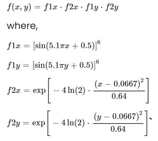
%CREATING A FUNCTION OF STALAGMITE

function[f] = stalagmite(input_vector)

 

        x = input_vector(1);  %Let the 1st input be x.

        y = input_vector(2);  %Let the 2nd input be y.

   

%By using the given functions in the challenge, we code it as below

f1x = (sin(5.1*pi*x + 0.5))^6;

f1y = (sin(5.1*pi*y + 0.5))^6;

 

f2x = exp((-4*log(2)*(x-0.0667).^2)/0.64);

f2y = exp((-4*log(2)*(y-0.0667).^2)/0.64);

 

f = -(f1x.*f1y.*f2x.*f2y);

end

 

%Since the GA algorithm of matlab generates a minima, the negative sign is

%inserted which denotes that the plot will be reversed and the stalagmite function

%created will be inversed to find the global maxima instead of minima.

 

Main Program:

Part1:

%Important Commands to clear the temporary memory, close all plots and

%clear the command window.

close all

clear all

clc

 

% Defining the search space from 0 to 0.6 with 150 equal intervals.

x = linspace(0,0.6,150);

y = linspace(0,0.6,150);

 

%To create a 2d mesh

%[xx,yy] = meshgrid(x,y)

%Assigning values to inputs

  for i = 1:length(x)  %Takes the values until length of xx

      for j = 1:length(y)  %Takes values until length of yy

          inputs(1) = x(i);

          inputs(2) = y(j);

          f(i,j) = stalagmite(inputs);

      end

  end

 

  iterations = 50; %creating a variable and assigning the number to which iterations

 performed

  %f = get_stalagmite(x,y);

 

 

 %Study case: 1

 tic % Starts the timer

 for z = 1:iterations % takes values until length of num_cases

         [inputs,fopt(z)]  = ga(@stalagmite,2);% solve stalagmite function using GA and

 assigning to variables

         xopt(z) = inputs(1);

         yopt(z) = inputs(2);

 end

 Timestudy_1 = toc; % Gives time taken to perform the study case.

 

 %Plotting

 figure(1)

 subplot(2,1,1) % Creates a sub plot in the figure

 hold on

 surfc(x,y,-f) % Creates a surface

 shading interp % Varies the color in each line segment and face by interpolating the

 colormap index or true color value across the line or face.

 plot3(xopt,yopt,-fopt,'marker','o','markersize',5,'markerfacecolor','r')% Plot3 command

 is used to plot in 3 axis

 % marker is used to create a visible points on the plot

 title('Unbounded Inputs') %Creates a title for the figure.

 xlabel('X Axis')

 ylabel('Y Axis')

 zlabel('Z Axis')

 subplot(2,1,2) %Subplot command is used to plot the figure in the same figure window.

 plot(-fopt)

 xlabel('Iterations')

 ylabel('Function Maximum')

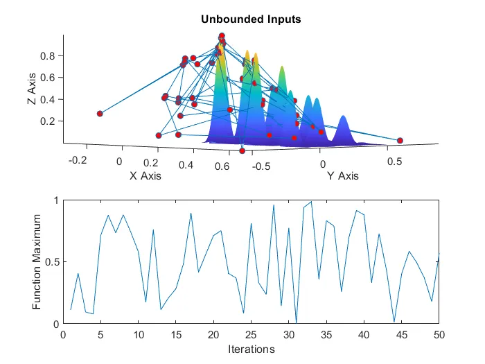
Output Obtained is as follows:

PART 2:

% Study Case 2: Studying between upper and lower bounds

tic

 for z = 1:iterations

         [inputs,fopt(z)] = ga(@stalagmite,2,[],[],[],[],[0;0],[0.4;0.4]);

         %defines a set of lower and upper bounds on the design variables

         xopt(z) = inputs(1);

         yopt(z) = inputs(2);

 end

 Timestudy_2 = toc;

 

 %Plotting

 figure(2)

 subplot(2,1,1)

 hold on

 surfc(x,y,-f)

 shading interp

 plot3(xopt,yopt,-fopt,'marker','o','markersize',5,'markerfacecolor','r')

 title('Bounded Inputs')

 xlabel('X Axis')

 ylabel('Y Axis')

 zlabel('Z Axis')

 subplot(2,1,2)

 plot(-fopt)

 xlabel('Iterations')

 ylabel('Function Maximum')

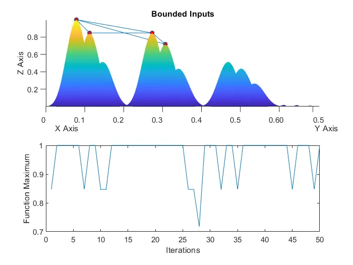
Output for the above is as follows:

PART 3:

% Study Case 3: Studying with a population size with increased GA interations.

 options = optimoptions('ga'); %returns a set of default options for the SolverName solver.

 options = optimoptions(options,'PopulationSize',300);  % Defining population size

 

 tic

 for z = 1:iterations

         [inputs,fopt(z)]  = ga(@stalagmite, 2,[],[],[],[],[0;0],[0.4;0.4],[],[],options);

         % Takes the values of options and solves ga in required population.

         xopt(z) = inputs(1);

         yopt(z) = inputs(2);

 end

 Timestudy_3 = toc;

 

 %Plotting

 figure(3)

 subplot(2,1,1)

 hold on

 surfc(x,y,-f)

 shading interp

 plot3(xopt,yopt,-fopt,'marker','o','markersize',5,'markerfacecolor','r')

 title('Increased Population Size')

 xlabel('X Axis')

 ylabel('Y Axis')

 zlabel('Z Axis')

 subplot(2,1,2)

 plot(-fopt)

 xlabel('Iterations')

 ylabel('Function Maximum')

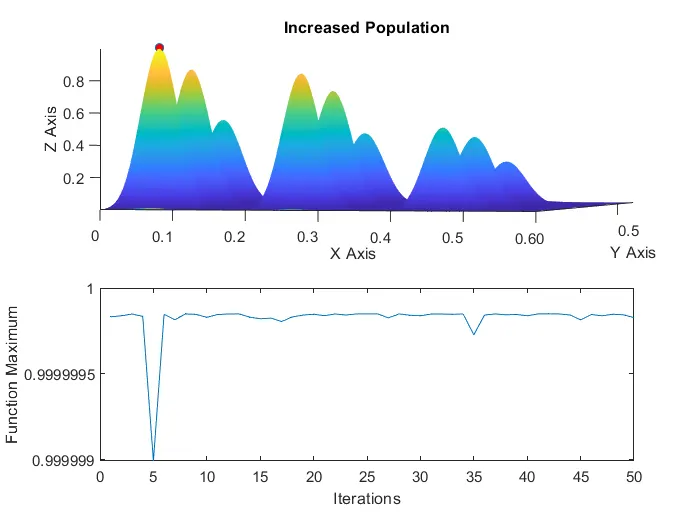
Output of the above is as follows:

To Find the value of Global Maximum Value, we code as follows:

GMV_1 = -(mean(fopt1));

GMV_2 = -(mean(fopt2));

GMV_3 = -(mean(fopt3));

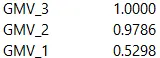
Here, GMV refers to global maximum value of the respecting parts as given above.

Explanation of 3 Parts of the Program:

Part 1: In this study, we have not set the limits and the obtained global maximum is for the whole search space.

Part 2: In this study, we have set the upper bound and lower bound limits to the study so that the global maximum is found between them.

Part 3: In this study, we have also added the the population size to fiind the global maximum using the optimoptions.

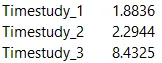
The Time study for the cases performed:

The Global Maximum Value for all 3 parts :