Week 3 - Solving second order ODEs

Introduction:

The 'ode45' is a versatile ODE solver and also solves non stiff differential equations. For differential equations with smooth solutions, ode45 is most accurate.

The following code is the function created using ode45.

function [dtheta_dt] = ode_func(t,theta,b,m,g,l);

 

theta1 = theta(1)

theta2 = theta(2)

dtheta1_dt = theta2

dtheta2_dt = -(b/m)*theta2 - (g/l)*sin(theta1)

 

[dtheta_dt] = [dtheta1_dt ; dtheta2_dt];

The above program is used in the main program to get the values. Therefore the code is as follows:

%To create an animated movie for a simple pendulum

 

%Important Commands

clear all

close all

clc

 

%Inputs for Pendulum

l = 1;           %length of the string

m = 1;           %mass of the ball in kg

b = 0.05;        %damping coefficient

g = 9.81;        %gravity in m/s^2

 

%Initial Conditions

theta_0 = [0;3];     %Angular displacement=0 & Angular Velocity=3.              

 

%Let us take timespan of 20 seconds

tspan = linspace(0,20,200);

 

%Solving the Differential Equation

[t,results] = ode45(@(t,theta) ode_func(t,theta,b,m,g,l),tspan,theta_0);

 

%Plotting the Damping Effect

figure(1)

hold on

plot(t,results(:,1),'linewidth',1.5); %time vs displacement

plot(t,results(:,2),'linewidth',1.5); %time vs angular velocity

xlabel('Time (secs)');

ylabel('Angular Displacement & Angular Velocity');

legend('Angular Displacement','Angular Velocity');

title('Damping Effect of a Simple Pendulum');

 

%Plotting  the Simple Pendulum with Animation

%Let ct be the counter, x0 and y0 be the initial points of the string i.e. the start point and let the x1 and y1 be the final points of the string i.e. the end points.

ct = 1;

for i = 1:length(results(:,1));

        x0 = 0;

        y0 = 0;

        x1 = l*sin(results(i,1));

        y1 = -l*cos(results(i,1));

 

%Creating a plot for the pendulum

figure(2)

plot([-0.5 0.5], [0 0],'linewidth',2); %Plot for fixed line.

hold on

plot([x0 x1],[y0 y1],'linewidth',2); %Plot for the string

hold on

plot(x1,y1,'marker','o','markerfacecolor','r','markersize',15); % %Plot for the ball

xlabel('Time Span (seconds)');

axis([-2 2 -2 2]);

title('Animation of a Simple Pendulum');

pause(0.03)

       

J(ct) = getframe(gcf)

ct = ct + 1;

hold off

end

 

%Creating an animated Movie for the pendulum

%Commands for the getting the movie file of the Simple Pendulum.

movie(J)

videofile = VideoWriter('Simple Pendulum Animation.avi','Uncompressed AVI'); 

open(videofile)

writeVideo(videofile,J)

close(videofile)

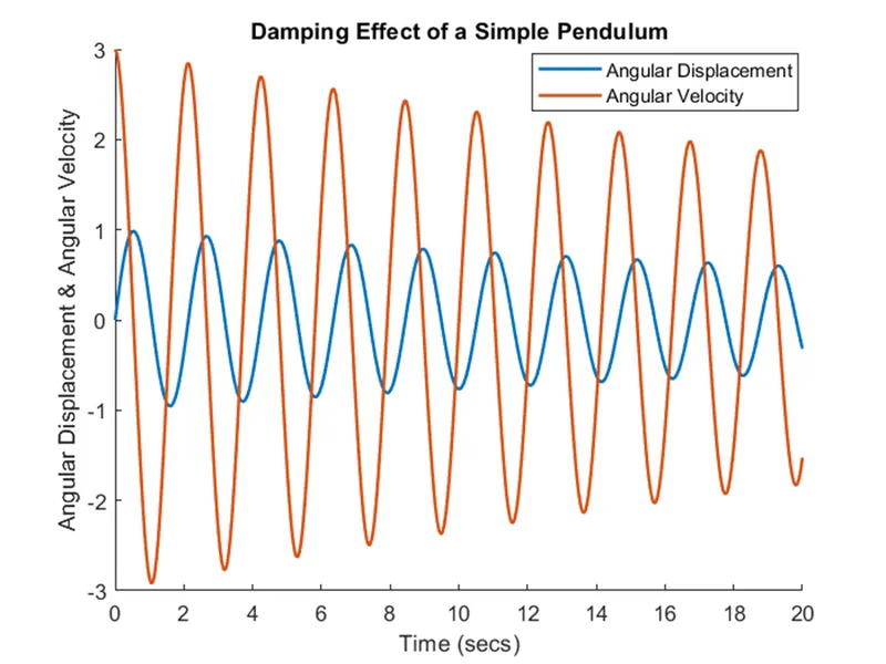
Following outputs are obtained:

Damping effect of the pendulum:

link to animation :https://drive.google.com/file/d/1zoZGEtL8pdVoz5-mXTtcVVcrvzt_1HYz/view?usp=sharing

Conclusion: Hence, we have succesfully studied the ode45 solver and also created an animated simple pendulum.