Week 4.1 - Genetic Algorithm

Program for stalagmite function.

function [f] = stalagmite(input_vector)
x = input_vector(1);
y = input_vector(2);
f1_x = (sin(5.1*pi*x + 0.5)).^6;
f1_y = (sin(5.1*pi*y + 0.5)).^6;
t1 = ((x-0.0667).^2)/(0.64);
f2_x = exp(-4.*log(2)*t1);
t2 = ((y-0.0667).^2)/(0.64);
f2_y = exp(-4.*log(2)*t2);
f = -(f1_x.*f2_x.*f1_y.*f2_y);
end

Program for 3-study and for plot maximum value and iteration

clear all
close all
clc

x=linspace(0,0.6,150);
y=linspace(0,0.6,150);
[xx,yy]=meshgrid(x,y);

for i=1:length(xx)
for j=1:length(yy)
input_vector(1)=xx(i,j);
input_vector(2)=yy(i,j);
f(i,j)=stalagmite(input_vector);
end
end
surfc(xx,yy,f)
%statistical behavior(unbounded) study-1
tic for study of time
num_cases=50 for no. of iteration
for i=1:num_cases
[input,fopt(i)]=ga(@stalagmite,2)
xopt(i)=input(1);
yopt(i)=input(2);
end

study1_time=toc
figure(1)
subplot(2,1,1)
hold on
surfc(xx,yy,-f)
shading interp
plot3(xopt,yopt,-fopt,'Marker','o','MarkerSize',5,'MarkerFaceColor','r')
title('unbounded input')

plot(-fopt)
xlabel('iteration')
ylabel('function maximum')

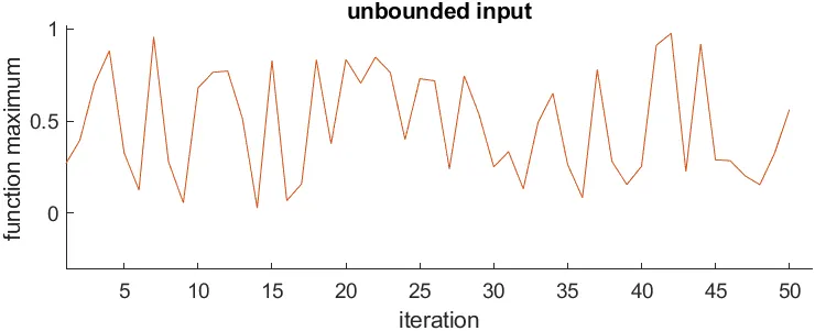
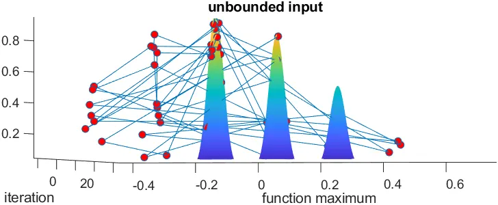
%study-2 statistical behavior with uper and lower bound
tic
for i=num_cases
[input,fopt(i)]=ga(@stalagmite,2,[],[],[],[],[0;0],[1;1]);
xopt(i)=input(1);
yopt(i)=input(2);
end
study2_time=toc
figure(2)
subplot(2,1,1)
hold on
surfc(xx,yy,-f)
shading interp
plot3(xopt,yopt,-fopt,'Marker','o','MarkerSize',5,'MarkerFaceColor','r')
title('bounded input')
subplot(2,1,2)

plot(-fopt)
xlabel('iteration')
ylabel('function maximum')

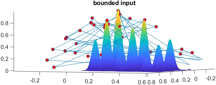
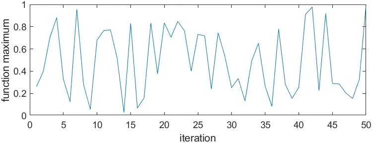
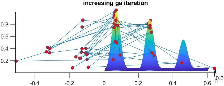
% study-3 increasing GA
options=optimoptions('ga');
options=optimoptions(options,'PopulationSize',300);
tic
for i=num_cases
[input,fopt(i)]=ga(@stalagmite,2,[],[],[],[],[0;0],[1;1],[],[],options);
xopt(i)=input(1);
yopt(i)=input(2);
end
study3_time=toc
figure(3)
subplot(2,1,1)
hold on
surfc(xx,yy,-f)
shading interp
plot3(xopt,yopt,-fopt,'Marker','o','MarkerSize',5,'MarkerFaceColor','r')
title('increasing ga iteration')
subplot(2,1,2)

plot(-fopt)
xlabel('iteration')
ylabel('function maximum')

Program for more accurate results of maximum value

clear all
close all
clc

x=linspace(0,0.6,150);
y=linspace(0,0.6,150);
[xx,yy]=meshgrid(x,y);

for i=1:length(xx)
for j=1:length(yy)
input_vector(1)=xx(i,j);
input_vector(2)=yy(i,j);
f(i,j)=stalagmite(input_vector);
end
end
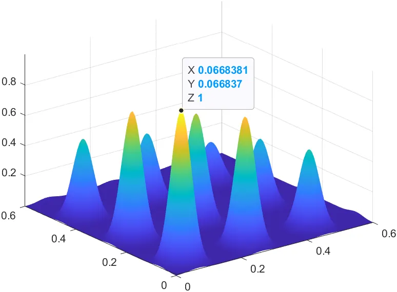
surfc(xx,yy,-f)
shading interp
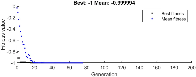
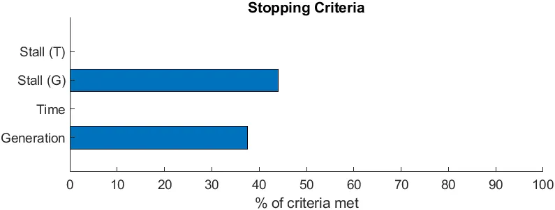
options=optimoptions('ga','PlotFcn',{@gaplotbestf,@gaplotstopping},'populationsize',170);
[x,fval]=ga(@stalagmite,2,[],[],[],[],[0;0],[1;1],[],options)
xopt=x(1);
yopt=x(2);
figure(1)
hold on

plot3(xopt,yopt,-fval,'ro','markersize',5,'markerfacecolor','r')

Genetic algorithm

genetic algorithm is a search based optimisation technique based on the principles of genetics and natural selection, and is inspired by Charles Darwin's theory of natural evolution

it is used to solve optimisation problems and machine learnings,

How GA works

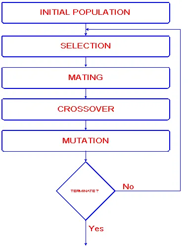
1. SELECTION-

in this step, the parents are selected from the sample data points, the main objective of the selection process is to select the highly fit individual.

the fitness value of given function will be compited ,the fitted value have most probability.

2. CROSS-OVER/MATING- in this process interchanging of genes takes place.

3.MUTATION-in this process the genes will be replaced by some random genes.

SYNTAX

x = ga(fun,nvars) here nvars-no. of design variable, used for finds a local unconstrained minimum
x = ga(fun,nvars,A,b) - find local minima subject to the linear inequalities
x = ga(fun,nvars,A,b,Aeq,beq)- find local minima subject to the linear equalities
x = ga(fun,nvars,A,b,Aeq,beq,lb,ub)- used defines a set of lower and upper bounds on the design variables, lb (lower bound) ub (uper bound)
x = ga(fun,nvars,A,b,Aeq,beq,lb,ub,nonlcon)
x = ga(fun,nvars,A,b,Aeq,beq,lb,ub,nonlcon,options)
x = ga(fun,nvars,A,b,[],[],lb,ub,nonlcon,IntCon)
x = ga(fun,nvars,A,b,[],[],lb,ub,nonlcon,IntCon,options)
x = ga(X) -finds the minimum for X
[x,fval] = ga(_)-fval, the value of the fitness function at x
[x,fval,exitflag,output] = ga(_)
[x,fval,exitflag,output,population,scores] = ga(_)