Week 4.1 - Genetic Algorithm

Selection(Genetic algorithm): During each successive generation, a portion of the existing population is selected to breed a new generation. Individual solutions are selected through a fitness-based process, where fitter solutions (as measured by a fitness function) are typically more likely to be selected. Certain selection methods rate the fitness of each solution and preferentially select the best solutions. Other methods rate only a random sample of the population, as the former process may be very time-consuming.

Genetic operators: Crossover and Mutation

The next step is to generate a second generation population of solutions from those selected through a combination of genetic operators: crossover (also called recombination), and mutation.

For each new solution to be produced, a pair of "parent" solutions is selected for breeding from the pool selected previously. By producing a "child" solution using the above methods of crossover and mutation, a new solution is created which typically shares many of the characteristics of its "parents". New parents are selected for each new child, and the process continues until a new population of solutions of appropriate size is generated. Although reproduction methods that are based on the use of two parents are more "biology inspired", some research suggests that more than two "parents" generate higher quality chromosomes.

These processes ultimately result in the next generation population of chromosomes that is different from the initial generation. Generally, the average fitness will have increased by this procedure for the population, since only the best organisms from the first generation are selected for breeding, along with a small proportion of less fit solutions. These less fit solutions ensure genetic diversity within the genetic pool of the parents and therefore ensure the genetic diversity of the subsequent generation of children.

ga syntax explanation:

The format for writing genetic algorithm in matlab is as follows:

f_min = ga(@function,nvars,A,B,Aeq,Beq,LB,UB,nonlcon,intcon,options)

Where,

- f_min = Local minima point.

- @function is the function to be called i.e stalagmite function

- nvars indicates the no. of variables used.

- A and B are used to indicate any kind inequalities that exist in the function.

- Same goes with Aeq and Beq.

- LB = lower bound.

- UB = upper bound.

- nonlcon gives two vectors representing inequalities and equalities.

- options is used to perform additional operations like increasing population size. This is done with the help of optimooptions

Code in MATLAB to optimise the stalagmite function and find the global maxima of the function.

clear all
close all
clc


% Defining the limits and spaces in between the limits
x = linspace(0,0.6,150);
y = linspace(0,0.6,150);
[xx, yy] = meshgrid(x,y);


% Introduction of the for loop
for i = 1 : length(xx)
 for j = 1 : length(yy)
 input_vector(1) = xx(i,j);
 input_vector(2) = yy(i,j);
 f(i,j) = stalagmite(input_vector);
 end
end


% Defining the 1st iteration to study the statistical behaviour
iterations = 50;
tic
for i = 1 : iterations
[inputs , f_optimum(i)] = ga(@stalagmite,2);
x_optimum(i) = inputs(1);
y_optimum(i) = inputs(2);
optimum_f(i) =  -f_optimum(i)
end
iteration_1_time = toc
% Plotting the data
figure (1)
subplot(2,1,1)
hold on
surfc(xx,yy,f)
shading interp
plot3(x_optimum,y_optimum,f_optimum,'marker','o','markersize',5,'markerfacecolor','r')
title('Unbounded Inputs')
subplot(2,1,2)
plot(f_optimum)
xlabel('Iterations')
ylabel('Function Maximum')


% Defining the 2nd iteration by proving upper and lower limits
iterations = 100;
tic
for i = 1:iterations
[inputs , f_optimum(i)] = ga(@stalagmite,2,[],[],[],[],[0;0],[1;1]);
x_optimum(i) = inputs(1);
y_optimum(i) = inputs(2);
optimum_f(i) =  -f_optimum(i)
end
iteration_2_time = toc
% Plotting the data 
figure (2)
subplot(2,1,1)
hold on
surfc(xx,yy,f)
shading interp
plot3(x_optimum,y_optimum,f_optimum,'marker','o','markersize',5,'markerfacecolor','r')
title('Bounded Inputs')
subplot(2,1,2)
plot(f_optimum)
xlabel('Iterations')
ylabel('Function Maximum')


% Defining the 3rd iteration for increasing the size of population
iterations = 150;
options = optimoptions('ga');
options = optimoptions(options,'populationsize',400)
tic
for i = 1 : iterations
[inputs , f_optimum(i)] = ga(@stalagmite,2,[],[],[],[],[0;0],[1;1],[],[],options);
x_optimum(i) = inputs(1);
y_optimum(i) = inputs(2);
optimum_f(i) = -f_optimum(i)
end
iteration_3_time = toc
%plotting
figure (3)
subplot(2,1,1)
hold on
surfc(xx,yy,f)
shading interp
plot3(x_optimum,y_optimum,f_optimum,'marker','o','markersize',5,'markerfacecolor','r')
title('Bounded inputs with modified population size')
subplot(2,1,2)
plot(f_optimum)
xlabel('Iterations')
ylabel('Functiosn Maximum')

Explanation for the above code:

1) Initially the search space required to execute the program using linspace command is defined which varies from 0 to 0.6 with 150 divisions in between.
2) Using the meshgrid command, row vectors x and y are converted into matrices xx and yy.
3) With the help of the for loop, the input vectors required for a stalagmite function are defined using the matrices xx and yy.
From here onwards, whole program is divided into three iterations whic produce the results as follows,

Iteration no. 1:

1) In the 1st iteraion, the behaviour of the algorithm is studied by not defining the limits. The ga command does not run within a particular searchspace, since we have not defined bounds.

2) For this we initially introduce a for loop within which we introduce a ga with stalagmite function with no limits defined. We store the results in a couple of arrays named inputs and f_optimum(i). We also use tic and toc who records the current time, and uses the recorded value to calculate the elapsed time respectively.

3) Eventually we plot the data using shading interp command which smoothens the visual by removing out the lines on the of the surface of the visual. Followed by that we conclude the first iteration by defining title, xlabel and ylabel.

The result of the above iteration is plot as follows,

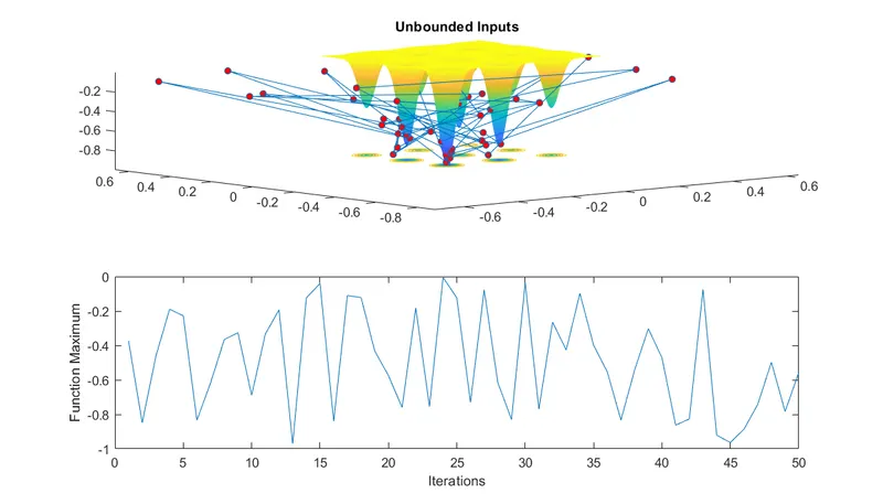
4) In the above image it can be explicitly seen that since the inputs are boundless ga command has mapped local maxima points outside our stalagmite function which is extremely undesirable. Also we cannot infer a particular value of global maxima from the above graph, and it is hence pointless. Moreover the study time is very less as the ga command is made only to run for 50 iterations.

Iteration no. 2:

1) This iteration is more or less identical to the first iteration, only here the bounds are stated i.e the lower and upper bounds are defined so as to know the boundaries within which the global maxima lies.

2) The plot for the 2nd iteration is as follows,

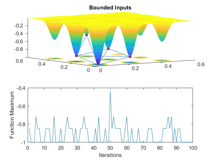
The above graph seems more clear and optimised as compared to that of the 1st iteration's graph, since here the bounds were defined and we could get only the values within our range. We are now more clear on the range within which our maxima lies. Also we can find the co-ordinates of the maximas.

Iteration no. 3:

1) The allover code for the 3rd iteration also stays same as the above two codes, only here the population size is increased so as to converge to the global maxima. For doing so we use optimoptions command to mention the population using 'PopulationSize' as an input which we have stated as 400.

2) Apart from this there are no changes in the code for 3rd iteration.

3) The graph for the 3rd iteration is as follows,

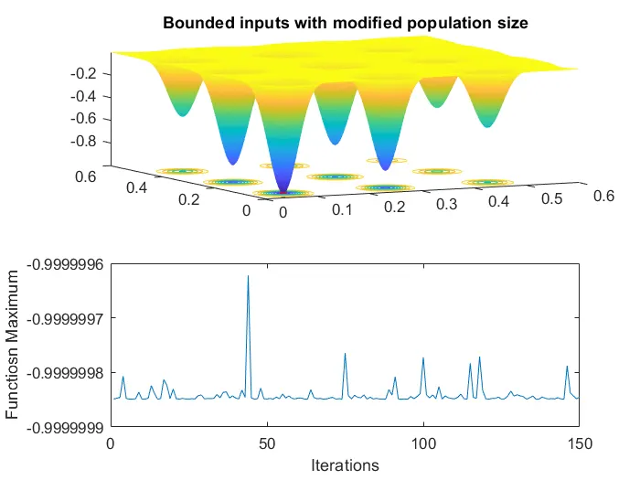
In this case we are getting the optimised value of global maxima with accurate range, since we increased the number of iterations and population size. Since the number of iterations and population size is increased the study time is so high compared to the previous two iterations. Also ga command gives more accurate results in case of bounded inputs and by increasing the number of iterations andpopulation size. It can also be stated that even if we define a particular search space for ga command, the ga command does not run inside the search space. Only in cases of bounded inputs we can get interfereable results.

Below is the stalagmite function code:

function [f] = stalagmite(input_vector)
x = input_vector(1);
y = input_vector(2);
f1 = (sin(5.1 * pi * x + 0.5)).^6 ;
f2 = exp(-4 * log(2) * ((x - 0.0667).^2)./0.64) ;
f3 = (sin(5.1 * pi * y + 0.5)).^6 ;
f4 = exp(-4 * log(2)*((y - 0.0667).^2)./0.64) ;
f = -(f1 * f2 * f3 * f4);
end 

Explanation for the stalagmite function:

1) A stalagmite function generally refers to the function with which we are generating values over a stalagmite kind of surface for finding out the local and global maxima and minima of that particular given function.The above function defines the stalagmite function which will be used in the main function.
2) The input vectors 'x' and 'y' will be assigned as per thr required values in the main function.
3) Negative sign used in the last line is to maximize the stalagmite function.

Conclusion: We can explicitcly draw out from the above 1st iteration that if we do not provide the bounds or limits in the ga command then the ga command has mapped local maxima points outside our stalagmite function, which is totally unexpected (Unbounded Inputs). In the 2nd iteration, we provided the bounds and we got a graph which was more clear and compact to visualize (Bounded Inputs). Eventually if we go through the 3rd iteration we can observe that when we increase the no. of iterations along with providing bounds and the population, we are getting the optimised value of global maxima with accurate range, since we increased the number of iterations and population size. Since the number of iterations and population size is increased the study time is so high compared to the previous two iterations (Bounded inputs with modified population size). Also we can get the iteration timings or study timings of the iterations 1, 2 and 3 to be 4.2124, 11.5390 and 102.5968 respectively from the computions which we have done.

No errors were encountered by me.