Simulation of a pendulum's motion using MATLAB.
AIM: To write a program in MATLAB that will simulate the pendulum motion.
OBJECTIVES OF THE PROJECT: To write a program that solves the following ODE. This ODE represents the equation of motion of a simple pendulum with damping.

Where,
g = gravity in m/s^2
L = length of the pendulum in m
m = mass of the ball in kg
b = damping coefficient
GOVERNING EQUATIONS: In Engineering, ODE is used to describe the transient behavior of a system. A simple example is a pendulum. The way the pendulum moves depends on the Newton’s Second Law of Motion. When this law is written down, we get a Second Order Ordinary Differential Equation that describes the position of the "ball" w.r.t time. The second order differential equation can be deriverd as follows;
According to the Newton’s Second Law of Motion,
`F=m × a
τ=I × α
-mg ×sinθ=m ×L^2 (d^2 θ)/〖dt〗^2
Assuming damping force is directly proportional to velocity,
-b dθ/dt - mg ×sinθ=m × L^2 (d^2 θ)/〖dt〗^2
b dθ/dt + mg ×sinθ + m × L^2 (d^2 θ)/〖dt〗^2 =0
Assuming θ= θ_1 so, dθ/dt= (dθ_1)/dt 〖 = θ〗_2
(dθ_2)/dt+ b/m 〖 ×θ〗_2+ g/l × sin〖θ_1 〗`
For simplicity we can convert this into matrix form which will make it solve in MATLAB,
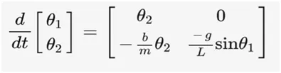
This is how we can reduce a Second Order Differential equation into a couple of First Order Differential equations.
BODY OF THE CONTENT: A simple gravity pendulum is an idealized mathematical model of a real pendulum. This is a weight (or bob) on the end of a massless cord suspended from a pivot, without friction. Since in this model there is no frictional energy loss, when given an initial displacement it will swing back and forth at a constant amplitude. The model is based on these assumptions;
- The rod or cord on which the bob swings is massless, inextensible and always remains taut.
- The bob is a point mass.
- Motion occurs only in two dimensions, i.e. the bob does not trace an ellipsebut an arc.
- The motion does not lose energy to frictionor air resistance.
- The gravitational field is uniform.
- The support does not move.
We can simulate the pendulum motion by considering all the parameters mentioned above. Program in MATLAB that will simulate pendulum motion is as follows;
% A program to solve 2nd order ODE
close all
clear all
clc

% Input parameters
b = 0.05
g = 9.81
l = 1
m = 1

% initial conditions
theta_o = [0;3]

%Time
time_span = linspace(0,20,1000);

%ODE function
[t, Results] = ode45(@(t,theta) pendulum_damped_ode(t,theta,b,m,g,l),time_span,theta_o);

%Plots
subplot(5,4,[13,14,17,18]);
plot(t,Results(:,1),'color','k');
hold on;
grid on;
plot(t,Results(:,2),'color','r');
xlabel('Time (sec)');
ylabel('Position and Angular Velocity');
hold off;
subplot(5,4,[15,16,19,20]);
plot(Results(:,1),Results(:,2));
xlabel('Position-Radians');
ylabel('Angular Velocity');
grid on;

%Animation of the pendulum
ct = 1;
for i = 1:length(Results(:,1))
 x0 = 0;
 y0 = 0;
 x1 = l * sin(Results(i,1));
 y1 = -l * cos(Results(i,1));
 subplot(5,4,[1,2,3,4,5,6,7,8,9,10,11,12]);
 plot([-l l],[0 0],'linewidth',4,'color','k');
 hold on;
 line([x0 x1],[y0 y1],'linewidth',2,'color','b');
 hold on;
 plot(x1,y1,'-o','markers',20,'markerfacecolor','r');

 grid on;
 axis([-1.5 1.5 -1.5 0.5]);
 pause(0.003);
 hold off;
 M(ct) = getframe(gcf);
 ct = ct + 1;
end


movie(M)
videofile = VideoWriter('Untitled_pendulum.avi','Uncompressed AVI');
open(videofile)
writeVideo(videofile,M)
close(videofile)
We also have to introduce a calling function pendulum_damped_ode in ode45 function;
function [dtheta_dt] = pendulum_damped_ode(t,theta,b,m,g,l)

 theta1 = theta(1);
 theta2 = theta(2);
 dtheta1_dt = theta2;
 dtheta2_dt = -(b/m)*theta2 - (g/l)*sin(theta1);
 dtheta_dt = [dtheta1_dt;dtheta2_dt];

end
EXPLANATION OF THE CODE: 1) First we define input parameters such as damping coefficient, gravity, length and mass which are all constant values.
2) A time matrix is also assigned from 0 to 20 s with 1000 points between them.
3) The time and results (Position and Angular Velocity) are calculated using the ode45 function. ode45 function in MATLAB is an inbuilt function which helps us in solving the ordinary differential equations. We store the results from ode45 function in an array consisting of t i.e time and results. We have created a function within ode45 function named pendulum_damped_ode, which consists of all the inputs which are defined initially.
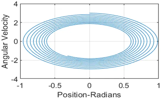
4) Next step is to plot Position alongside Angular Velocity and after that we give xlabel, ylabel and all other parameters.
5) Then for animation purpose, we use ct, the counter to count the no. of frames. Next step is to use for loop with marking the co-ordinates using sin and cos functions.
6) Then we plot the animation with the help of plot command by using different linewidths, markers, colors etc. Then eventually we on the grid, specify the axes limits and by defining a pause of 0.003 we then use getframe command to get the frames accordingly, after each frame we count it and increase it by adding 1 to the counter. Lastly we end the for loop.
7) Then for making a movie and saving it we use movie command, we have to mention the file name and the movie format for saving the video by giving it an extension of '.avi'.
8) We finally conclude the code by giving commands to start and end the code.
OUTPUT: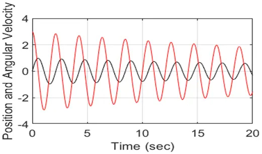
Link for animation of motion of the pendulum.
CONCLUSION: There are hundreds of ODEs that describe key phenomena and if you have the ability to solve these equations then you will easily be able to simulate any of these systems by using MATLAB in an efficient way. That’s the kind of ability MATLAB has.