Week 4.1 - Genetic Algorithm
function [f] = stalagmite(input_vector) % stalagmite call functions
x = input_vector(1);
y = input_vector(2);
f1_x = (sin(5.1*pi*x + 0.5))^6;
f1_y = (sin(5.1*pi*y + 0.5))^6;
f2_x = exp(-4.*log(2)*((x-0.0667)^6)/(0.64));
f2_y = exp(-4.*log(2)*((y-0.0667)^6)/(0.64));
f = -(f1_x.*f2_x.*f1_y.*f2_y); % minus sign (-) shows that for finding the largest value of functions
end
clear
close all
clc
% space function
x=linspace(0,0.5,50);% x-coordinate
y=linspace(0,0.5,50); %y-coordinate
[xx,yy]=meshgrid(x,y);%2D matrix formation
num_cases=50; %iteration function
% Stalagmite function formation
for i=1:length(xx)
for j=1:length(yy)
input_vector(1)=xx(i,j);
input_vector(2)=yy(i,j);
f(i,j)=stalagmite(input_vector); %values of function in given search space
end
end
surfc(xx,yy,-f); % 3D surface generation
shading interp % To remove the grid lines produced by the mesh grid
xlabel('x')
ylabel('y')
zlabel('z')
% Study 1
tic % time taken for execution
for i=1:num_cases
[inputs,fopt(i)]=ga(@stalagmite,2); %calculating optimal value functions
xopt(i)=inputs(1);
yopt(i)=inputs(2);
end
study1_time=toc
figure(1)
subplot(2,1,1)
surfc(xx,yy,-f);
hold on
shading interp
plot3(xopt,yopt,-fopt,'marker','o','markersize',5,'markerfacecolor','r');
xlabel('x');
ylabel('y');
grid on
subplot(2,1,2)
plot(-fopt);
xlabel('iterations')
ylabel('opt value')
% Study 2
tic
for j=1:num_cases
[inputs,fopt(j)]=ga(@stalagmite,2,[],[],[],[],[0;0],[1;1]); % [0;0],[1;1] lower and upper limit for optimal values
xopt(j)=inputs(1);
yopt(j)=inputs(2);
end
study2_time=toc
%PLOTTING
figure(2)
subplot(2,1,1)
hold on
surfc(xx,yy,-f)
shading interp
plot3(xopt,yopt,-fopt,'marker','o','markersize',5,'markerfacecolor','r');
xlabel('x');
ylabel('y');
grid on
subplot(2,1,2)
plot(-fopt);
xlabel('iterations')
ylabel('opt value')
%Study 3
options=optimoptions('ga','populationsize',50000) %increasing population size
tic
for k=1:num_cases
[inputs,fopt(k)]=ga(@stalagmite,2,[],[],[],[],[0;0],[1;1],[],[],options);
xopt(k)=inputs(1);
yopt(k)=inputs(2);
end
study3_time=toc
%PLOTTING
figure(3)
subplot(2,1,1)
hold on
surfc(xx,yy,-f)
shading interp
plot3(xopt,yopt,-fopt,'marker','o','markersize',5,'markerfacecolor','r');
xlabel('x');
ylabel('y');
grid on
subplot(2,1,2)
plot(-fopt);
xlabel('iterations')
ylabel('opt value')
gentic algorthim syntax in MATLAB
OUTPUT
Figure 1 shows the stalagmite plot developed in Matlab. In order to find the maximum value f, the minus sign(-) is inserted in the function c because by default the genetic algorithm used in Matlab was developed for finding the minimum value. From Figure 2 it is understood that for each iteration there are many optimum values, which does not show any constant optimum value and these results cannot be considered as a solution. In order to reduce the fluctuation in the optimum value, 'GA' syntax was added with the upper and lower bound value as 0 to 1 and their results are shown in Figure 3. This study showed a fluctuation during the iteration and these results cannot be considered. Further to reduce the fluctuation the population is increased from 170 to 1000 and found a fluctuation between two different optimum points as shown in Figure 4. To reduce the fluctuation the population was increased from 1000 to 2000 and found an optimum value of x=0.068 and y=0.068 with a function value of f=-1
t1
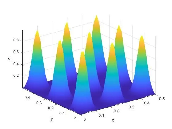
Figure 1 stalagmite plot in the MATLAB
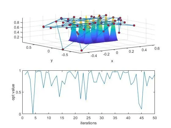
Figure 2 Genetic algorithm optimization for study 1
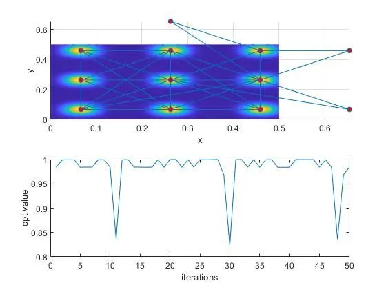
Figure 3 Genetic algorithm for study 2 through making optimum values within 0 to 1.
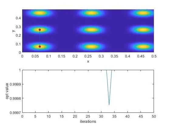
Figure 4 Genetic algorithm performed by increasing population to 1000
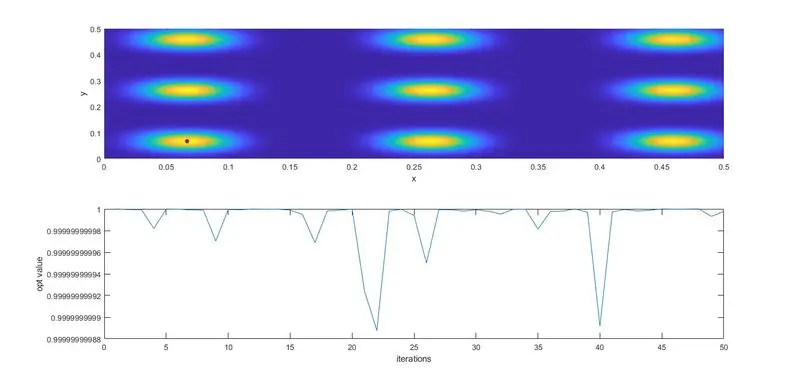
Figure 5 Genetic algorithm performed by increasing population from 1000 to 2000
About GENETIC ALGORITHMS (GA)
Genetic algorithms depend on biologically inspired operators including mutation, crossover, and selection to develop high-quality solutions to optimization and search problems.
vARIOUS PHASES IN GA-
- POPULATION INITIALIZATION
- Fitness Function 1. fitness values are used for the reproduction of the children.1. Selection
The idea of the selection phase is to select the fittest individuals and let them pass their genes to the next generation.
3. Reproduction
Generation of offspring happen in 2 way:
Crossover
a random point is selected while mating a pair of parents to generate offspring.
Mutation
Crossover
a random point is selected while mating a pair of parents to generate offspring.
There are 3 major types of crossover.
Single Point Crossover:
A point on both parents’ chromosomes is picked randomly, and designated a ‘crossover point’.
Two-Point Crossover: Two crossover points are picked randomly from the parent chromosomes.
Unifofm Crossover: In a uniform crossover, typically, each bit is chosen from either parent with equal probability
B) Mutation
Mutation happens to take care of diversity among the population and stop premature convergence.