Project 2 - Rankine cycle Simulator
clear all
clc
close all
%given data
p1=30; % inlet Turbine pressure
T1=400; % inlet turbine temperature
p2=0.05; % outlet turbine pressure
%state 1
h1=XSteam('h_pT',p1,T1); %Enthalpy at state 1
s1=XSteam('s_pT',p1,T1); % Entropy temperature at state 1
Tsat1=XSteam('Tsat_p',p1);%Saturation Temp.at p1
hg1=XSteam('hV_p',p1); % saturated vapor enthalpy at p1
hf1=XSteam('hL_p',p1);% saturated liquid enthalpy at p1
sg1=XSteam('sV_p',p1);% saturated gas entropy at p1
sf1=XSteam('sL_p',p1);% saturated gas entropy at p1
%state 2
s2=s1 % isentropic expansion
sf2=XSteam('sL_p',p2);% saturated gas entropy at p2
sg2=XSteam('sV_p',p2);% saturated gas entropy at p2
x2=(s2-sf2)/(sg2-sf2);% vapor fraction at state
hg2=XSteam('hV_p',p2);% saturated vapor enthalpy at p2
hf2=XSteam('hL_p',p2);% saturated liquid enthalpy at p2
h2=hf2+(x2*(hg2-hf2));% Enthalpy at state 2
%state 3
p3=p2 % constant pressure heat removal
s3=XSteam('sL_p',p3); %entropy at state 3
h3=XSteam('hL_p',p3); % enthalpy at state 4
% state 4
s4=s3;%entropy at state4
p4=p1; %pressure at state 4
%work done by the turbine
W_T=h1-h2 % workdone by the turbine
%work done by the pump
v3=XSteam('vL_p',p3); %specific volume
W_P=v3*(p4-p3)*100;%work done by the pump
h4=h3-W_P; %Enthalpy at state 4
W_net=W_T-W_P; % net workdone by the rankine cycle
Q_in=h1-h4; %heat addition
Q_out=h2-h3; %heat rejection
T_efficiency=(W_net/Q_in)*100;% thermal efficiency
sp_s=(3600/W_net);%steam consumption rate
BWR=W_P/W_T;
T3=XSteam('Tsat_p',p3);
T2=T3;
Cp4=XSteam('Cp_ps',p4,s4);
Cv4=XSteam('Cv_ps',p4,s4);
k=Cp4/Cv4
%temperature at state point4
T4=T3/((p3/p4)^((k-1)/k))
T6=XSteam('Tsat_p',p1);% temperature at state 6
s5=XSteam('sL_p',p1);% entropy at state 5
s6=XSteam('sV_p',p1);% entropy at state 6
h5=XSteam('hL_p',p1);% entalpy at state 5
h6=XSteam('hV_p',p1);% entalpy at state 6
T5=T6;
T=linspace(1,600,50000)
for i=1:length(T)
sf(i)=XSteam('sL_T',T(i));
sg(i)=XSteam('sV_T',T(i));
hf(i)=XSteam('hL_T',T(i));
hg(i)=XSteam('hV_T',T(i));
end
%T-S diagram
figure (1)
hold on
%% saturation curve line
plot(sf,T,'color','b','LineWidth',3)
plot(sg,T,'color','b','LineWidth',3)
%% s-T curve obtained plot from calcualtions
plot([s1 s2],[T1 T2],'linewidth',3)
plot([s2 s3],[T2 T3],'linewidth',3)
plot([s3 s4],[T3 T4],'linewidth',3)
plot([s4 s5],[T4 T5],'linewidth',3)
plot([s5 s6],[T5 T6],'linewidth',3)
s_1=linspace(s6,s1,100);
for j=1:length(s_1)
Tc(j)=XSteam('T_ps',p1,s_1(j));
end
plot(s_1,Tc,'color','r','LineWidth',3)
text(s1+0.3,T1,'1')
text(s2+0.3,T2,'2')
text(s3,T3-20,'3')
text(s5-0.5,T4+230,'4')
title('Entropy Curve')
xlabel('Entropy (kJ/kgK)', 'FontSize', 10)
ylabel('Temperature (degree-Celcius)', 'FontSize', 10)
legend('Saturation curve line')
%% h-s diagram
figure (2)
hold on
%% saturation curve line
plot(sf,hf,'color','b','lineWidth',2)
plot(sg,hg,'color','b','lineWidth',2)
%% h-s diagram obtained plot from calcualtions
plot([s1 s2],[h1 h2],'linewidth',2)
plot([s2 s3],[h2 h3],'linewidth',2)
plot([s3 s4],[h3 h4],'linewidth',2)
hc=linspace(h4,h5,1000)
for k=1:length(hc)
s_q=XSteam('s_ph',p1,hc(k))
end
plot(s_q,hc,'color','r','linewidth',2)
plot([s5 s6],[h5 h6],'color','r','linewidth',2)
for l=1:length(s_1)
h_c(l)=XSteam('h_ps',p1,s_1(l))
end
plot(s_1,h_c,'LineWidth',2)
text(s1+0.2,h1,'1')
text(s2+0.2,h2,'2')
text(s3,h3-120,'3')
text(s4,h4+120,'4')
title('Enthalpy VS Entropy')
xlabel('Entropy (kJ/kgK)', 'FontSize', 10)
ylabel('Enthalpy (kJ/kg)', 'FontSize', 10)
legend('Saturation curve line')
%% Results are displayed in the commend window
fprintf('%50s \r\n','Rankine Cycle Results')
fprintf('%21s %53s\r\n','At State point 1','At State point 2')
fprintf('%8s %8f %s %40s %8f %s \r\n','p1=',p1,'bar','p2=',p2,'bar')
fprintf('%8s %8f %s %29s %8f %s \r\n','T1=',T1,'degree-celcius','T2=',T2,'degree-celcius')
fprintf('%8s %8f %s %38s %8f %s \r\n','h1=',h1,'kJ/kg','h2=',h2,'kJ/kg')
fprintf('%8s %8f %s %40s %8f %s \r\n','s1=',s1,'kJ/kgK','s2=',s2,'kJ/kgK')
fprintf('%21s %53s\r\n','At State point 3','At State point 4')
fprintf('%8s %8f %s %40s %8f %s \r\n','p3=',p3,'bar','p4=',p4,'bar')
fprintf('%8s %8f %s %29s %8f %s \r\n','T3=',T3,'degree-celcius','T4=',T4,'degree-celcius')
fprintf('%8s %8f %s %38s %8f %s \r\n','h3=',h3,'kJ/kg','h4=',h4,'kJ/kg')
fprintf('%8s %8f %s %40s %8f %s \r\n','s3=',s3,'kJ/kgK','s4=',s4,'kJ/kgK')
fprintf('%45s %8f %s \r\n','Work done by the turbine=',W_T,'kJ/kg')
fprintf('%45s %8f %s \r\n','Work done by the pump=',W_P,'kJ/kg')
fprintf('%45s %8f %s \r\n','Thermal efficiency of the Rankine cycle=',T_efficiency,'percentage')
fprintf('%45s %8f \r\n','Steam consumption rate =',sp_s)
fprintf('%45s %8f \r\n','Back work ratio =',BWR)
OUTPUT:
Figure 1 and 2 shows the results displayed in the command window in Matlab. Figure 3 represent the temperature vs entropy. The simulation starts from 1 in which the isentropic process takes place with heat rejections. The steam from the outside of the turbine gets cooled in the condenser and became a saturated liquid. The saturated liquid from the pump is again sent into the boiler for the cyclic process.
Figure 4 represents the entropy vs enthalpy, from the relation it is understood that when heat is added to the system the entropy is increased and vice versa as the temperature is reduced the entropy is decreased considerably.
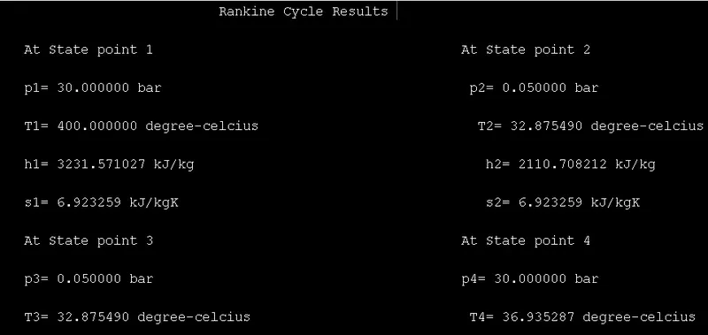
Figure 1 Rankine cycle results
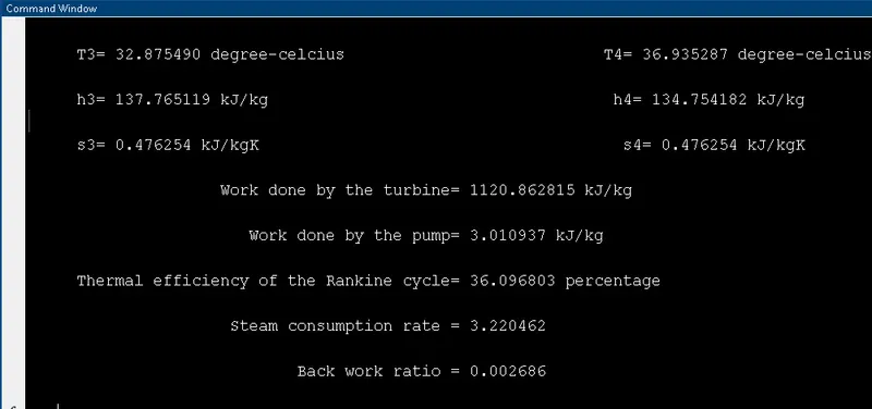
Figure 2 Rankine cycle results
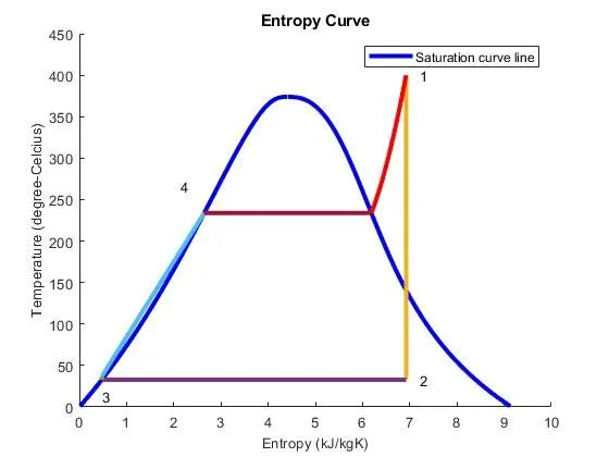
Figure 3 T VS S graph
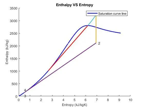
Figure 4 T VS S graph