Week 4.1 - Genetic Algorithm

what is stalagmite function?
The stalagmite function is a mathematical model that aids in the formation of local minima and peaks.
It's a three-dimensional function with a number of local maxima and minima and only one
global maximum or minimum because of the way it's created.
The term "stalagmite" refers to a sort of rock structure that emerges from a cave's floor.
Due to the buildup of debris deposited on the floor as a result of ceiling drippings, the cave has formed.

stalagmite program:-
%Define Stalagmite Function

function [f] = stalagmite(input_vector)
x = input_vector(1);
y = input_vector(2);

t1 = (sin((5.1*pi*x)+0.5))^6;
t2 = (sin((5.1*pi*y)+0.5))^6;
t3 = exp(-4*log(2)*((x-0.0667)^2)/0.64);
t4 = exp(-4*log(2)*((y-0.0667)^2)/0.64);

f = -(t1*t2*t3*t4);
end

prgoram :-
clear all
close all
clc

% search space
x = linspace(0,0.6,150);
y = linspace(0,0.6,150);
n = 50;

% creating a 2D mesh
[xx yy] = meshgrid(x,y);

% evaluating stalagmite function
for i = 1:length(xx)
for j = 1:length(yy)
input_vector(1)=xx(i,j);
input_vector(2)=yy(i,j);
f(i,j) = define_stalagmite(input_vector);
end
end

% study 1 : statstical behaviour

tic
for i = 1:n
[inputs,fopt(i)] = ga(@define_stalagmite,2);
xopt(i) = inputs(1);
yopt(i) = inputs(2);
end
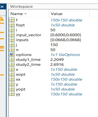
study1_time = toc

figure(1)
subplot(2,1,1)
hold on
surfc(xx,yy,-f)
shading interp
xlabel('x-axis')
ylabel('y-axis')
title('statistical behaviour with unbound inputs')
plot3(xopt,yopt,-fopt,'marker','o','markersize',5,'markerfacecolor','r')
subplot(2,1,2)
plot(-fopt)
xlabel('no. of iterations')
ylabel('function maximum')

% study 2 : statstical behaviour with upper and lower bounds

tic
for i = 1:n
[inputs,fopt(i)] = ga(@define_stalagmite,2,[],[],[],[],[0,0],[1;1]);
xopt(i) = inputs(1);
yopt(i) = inputs(2);
end

study2_time = toc

figure(2)
subplot(2,1,1)
hold on
surfc(xx,yy,-f)
shading interp
xlabel('x-axis')
ylabel('y-axis')
title('statistical behaviour with upper and lower bounds')
plot3(xopt,yopt,-fopt,'marker','o','markersize',5,'markerfacecolor','r')
subplot(2,1,2)
plot(-fopt)
xlabel('no. of iterations')
ylabel('function maximum')

% study3 : statstical behaviour with increasing iterations of GA

options = optimoptions('ga');
options = optimoptions(options,'populationsize',300);

tic
for i = 1:n
[inputs,fopt(i)] = ga(@define_stalagmite,2,[],[],[],[],[0,0],[1;1],[],[],options);
xopt(i) = inputs(1);
yopt(i) = inputs(2);
end

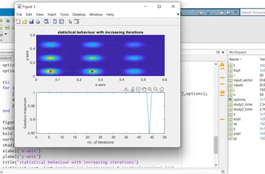
figure(3)
subplot(2,1,1)
hold on
surfc(xx,yy,-f)
shading interp
xlabel('x-axis')
ylabel('y-axis')
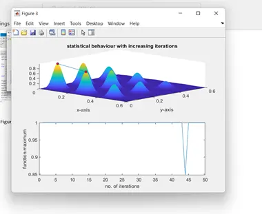
title('statistical behaviour with increasing iterations')
plot3(xopt,yopt,-fopt,'marker','o','markersize',5,'markerfacecolor','r')
subplot(2,1,2)
plot(-fopt)
xlabel('no. of iterations')
ylabel('function maximum')

whats in this program:-
1. Then, using the 'linspace' command, the 'X' and 'y' arrays are defined to construct values at 150 equal intervals.
2.Using the'meshgrid' command, a 2D mesh of x and y array is formed,
and the number of iterations or cases that the code should run is specified. n = 50 is the answer.
3. To evaluate the stalagmite function, a "for" loop is used,
with "' initialised and another "for" loop for each value of 'l'.
To initialise "", a loop is utilised.
4.The xx' and yy' input vector values are specified, as well as the stalagmite function for these input vectors.
This will result in a simple stalagmite function, which we may plot separately if necessary.
5.After preparing the function's inputs, the following step is to acquire the results for three genetic instances.
algorithm. The maximum value of a function is determined in the first case or study with no limits, boundaries, or constraints.
There are no restrictions.
6.This is accomplished using a 'for' loop in which we utilise the 'ga' syntax to provide values for inputs and the best maximum value.
The 'ga' syntax is used to call the stalagmite function, and the number of variables 'nvars' is two.
7. The 'tic' and 'toc' commands are used before and after each iteration to determine how long it takes to solve the loop for 50 iterations.
following the loop, respectively.
8.Using the'surf' command for xx, y, and function output, the function formed in the loop is displayed. To
The'shading interp' command is used to ignore the surface gridlines and get a smooth and clean graphic. The
'subplot (2,1,1)' is used to plot numerous plots on the same figure while also dividing
the graphic into a 2xl grid and allowing the axes to be moved around. positioned at 1

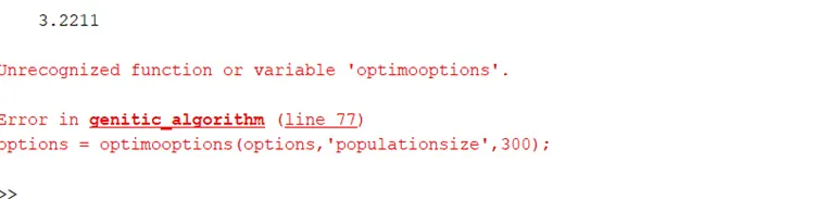
error caused due to spelling mistake :-

error caused due to @ sign was missing:-

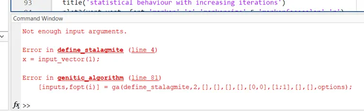
figure 1:- statistical behaviour with unbound inputs.

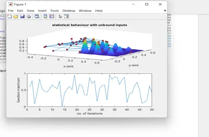
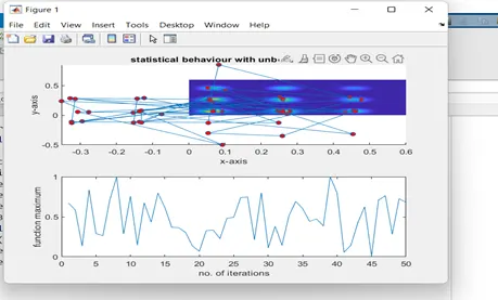
figure 2:- statstical behaviour witj upper and lower bounds

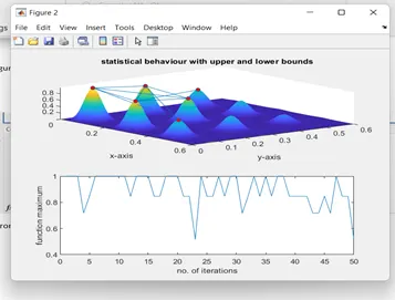
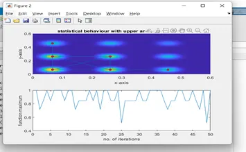
figure 3:- statistical behaviour with increasing iteration.

table