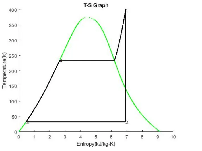
Project 2 - Rankine cycle Simulator

main program

clear all
close all
clc

disp(' RANKINE CYCLE SIMULATOR ');
disp('1-2 is Isentropic Expansion in the Turbine');
disp('2-3 is Constant Pressure Heat Rejection by the Condenser');
disp('3-4 is Isentropic Compression in the Pump") ;
disp('4-1 is Constant Pressure Heat Addition by the Boiler');
fprintf('n');

%Taking inputs from user
P1= input ('Enter the Pressure at the Turbine Inlet (in bar):’);
T1 = input ('Enter the Temperature at the Turbine Inlet (in Degree Celcius):’);
P2= input ('Enter the Pressure at the Condenser (in bar):’);

%calculating state values

%At state point 1
H1= XSteam('h pT', P1, T1) ;
S1 = xSteam('s pT' ,P1, T1);
H_L1 = xsteam('hL p' ,P1);
H_G1 = xsteam ('hv p' ,P1) ;
S_L1= XSteam('sL p',P1)；
S_G1 = Xsteam('sV p' ,P1);
T_satl= XSteam('Tsat p', P1) ;

%At state point 2
S2 = S1;
S_L2 = XSteam(' sL p, P2) ;
S_G2 = xSteam('sV p'‚P2) ;
D = (S2-S L2) / (S G2-S L2); %Calculating the dryness fraction
H_L2= XSteam("hL p'‚P2) ;
H_G2 = XSteam('hv p', P2) ;
H2 = H L2 + D* (H G2 - H L2); %Calculating the enthalpy at point 2
T2 = XSteam( 'T ph' , P2, H2) ;
T_ sat2 = XSteam('Tsat_p' , P2);

%At state point 3
p3 = P2;
T3= T2;
H3= H_L2;
S3= S_L2;
%At state point 4
P4=p1;
S4= S3;
T4 = XSteam ('T pS',P4, S4) ;
H4 = XSteam('H ps' ,P4, S4) ;

%Calculating Work, Back Work Ratio, Specific Steam Conductivity and Efficiency

%Turbine work
W_T = H1 -H2;

%Pump work
W_P=H4 - H3;

%Net work
W_NET = WT - WP;

%Thermal Efficiency of the Rankine Cycle
EFF = (W NET/(H1- H4) ) *100 ;

%Back Work Ratio
BWR = W_P/W_T;
%Specific Steam Conductivity
SSC = 3600/W_T;

%Displaying results
%state point 1
disp('. RESULTS. ‘);
disp('At State point 1');
fprintf('nP1 is : %.2f Bar n',P1);
fprintf('T1 is : %.2f Deg Celcius n', T1) ;
fprintf('H1 is : %.2f KJ/kg n' ,H1);
fprintf('S1 is : %.2f KJ/kgK nn' ,S1) ;

%Values of state point 2
disp('At State point 2');
fprintf ('nP2 is : %.2f Bar n' , P2) ;
fprintf('T2 is : %.2f Deg Celcius n' ,T2);
fprintf('H2 is : %.2f KJ/kg n', H2) ;
fprintf( 'S2 is : %.2f KJ/kgK nn', S2) ;

%Values of state point 3
disp(‘At State point 3');
fprintf('nP3 is : %.2f Bar n',P3) ;
fprintf('T3 is : %.2f Deg Celcius n', T3) ;
fprintf( 'H3 is : %.2f KJ/kg n' ,H3) ;
fprintf('S3 is : %.2f KJ/kgk nn',S3) ;

*Values of state point 4
disp('At State point 4') ;
fprintf('nP4 is : %.2f Bar n' ,PA) ;
fprintf(‘T4 is : %.2f Deg Celcius n', T4) ;
fprintf('H4 is : %.2f KJ/kg n', H4) ;
fprintf('S4 is : %.2f KJ/kgk n', S4) ;

%Turbine Work
fprintf('nTurbine work : %.2f KJ/kg n’,W_T);

%Pump work
fprintf( 'Pump work : %.2f KJ/kg n' ,W_P);

%Net Work
fprintf('Net work : %.2f KJ/kg n',W_NET) ;

%Thermal Efficiency
fprintf("thermal efficiency : %.2f %' ,EFF);

%Specific steam Conductivity
fprintf('specific steam Conductivity : %.2f kg/KWh n'', SSC);

%Back work ratio
fprintf('Back work Ratio is : %f n', BWR);

%plotting of T-S curve
t = linspace(0,373.5,200);
figure(1)
hold on

for i = 1:length(t)
plot (xsteam( 'sL_T' , t(i)) ,t(i), 'g.’)
plot(xSteam( 'sV_T' , t(i)) ,t(i), ‘g.’)
end

plot ([S1 S2],[T1 T2], 'linewidth',2, 'color', 'k')
text (S1, T1, ‘1' ,’Fontsize’,10)
if D>1
T3 = T_sat2;
plot([S2 S G2 S3 S4], [T2 T_sat2 T3 T4],'linewidth',2,'color', 'k')
T2 = T sat2;
text(S2, T2,’2', "Fontsize',10)
text (S3, T3, '3', 'Fontsize',10)
else
plot ([S2 S3 S4], [T2 T3 T4], 'linewidth', 2, 'color', 'k')
text (52, T2, '2', 'Fontsize',10)
text (53, T3, '3', 'Fontsize',10)
end

n= linspace(T1, T2, 500) ;
for i= 1:length(n)
plot (xsteam('s_pT',P1,n(i)),n(i),'.,'linewidth',2,'color','k’)
end

plot([S L1 S G1],[T_sat1 T_sat1],‘linewidth*, 2, 'color', 'k’)
text(S_L1,T sat1, '4','Fontsize',10)
×label(' Entropy(kJ/kg-K)
ylabel('Temperature(k)’)
title('T-S Graph' )

%Plotting of H-S Curve
figure(2)
hold on
for i = 1:length(t)
plot(xSteam('sL_T',t(i)),XSteam('hL_T',t(i)),"b.')
plot (xSteam('sV T',t (i)) ,XSteam ('hv T',t(i)), 'b.')
end
plot([S1 S2 S3 S4 S1],[H1 H2 H3 H4 H1] ‘linewidth' , 2, 'color',’k’)
text (S1,H1, '1' , 'Fontsize',10)
text (S2, H2, '2' , 'Fontsize', 10)
text (S3,H3, ' 3', ‘Fontsize,10)
text (S4, H4, ' 4' , 'Fontsize,10)
xlabel ('Entropy (kJ/kg-K)’)
label(' Enthalpy (kJ/kg)‘)
title('H-S Graph' )

command window

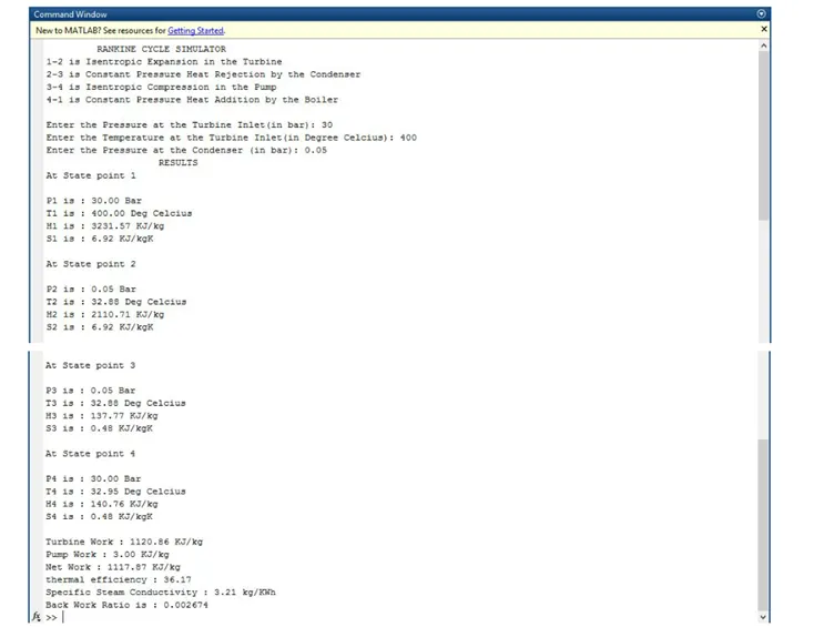
h-s graph

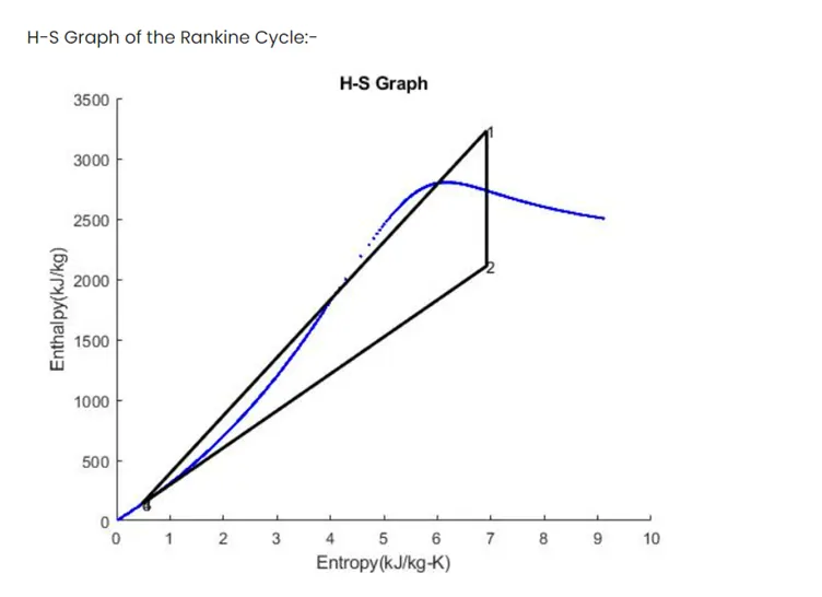
t-s graph