Week 4.1 - Genetic Algorithm

OBJECTIVE :- Writing a program to solve Global optimisation problem.

AIM :-

• ga_main :

  clear all
  close all
  clc
  
  % Defining our search space
  x = linspace(0,0.6,150);
  y = linspace(0,0.6,150);
  num_cases = 50;
  
  % Creating a 2Dimensional mesh
  [xx yy] = meshgrid(x, y);
  
  % Evaluating the stalagmite function
  for i = 1:length(xx)
      for j = 1:length(yy)
          input_vector(1)=xx(i,j);
          input_vector(2)=yy(i,j);
          f(i,j) = stalagmite(input_vector);
      end
  end
  tic
  % Study 1 - Satistical behaviour
  for i  = 1:num_cases
      [inputs, fopt(i)] = ga(@stalagmite, 2);
      xopt(i) = inputs(1);
      yopt(i) = inputs(2);
  end 
  
  study1_time = toc;
  
  figure(1)
  subplot(2,1,1)
  hold on
  surfc(x, y, f)
  shading interp
  plot3(xopt,yopt,fopt,'marker','o','markersize',5,'markerfacecolor','r')
  title('Unbounded inputs')
  subplot(2,1,2)
  plot(fopt)
  xlabel('Iterations')
  ylabel('Function minimum')
  
  tic
  % Study 2 - Statistical behaviour - with upper and lower bounds
  for i  = 1:num_cases
      [inputs, fopt(i)] = ga(@stalagmite, 2,[],[],[],[],[0;0],[1;1]);
      xopt(i) = inputs(1);
      yopt(i) = inputs(2);
  end 
  study2_time = toc;
  
  figure(2)
  subplot(2,1,1)
  hold on
  surfc(x, y, f)
  shading interp
  plot3(xopt,yopt,fopt,'marker','o','markersize',5,'markerfacecolor','r')
  title('Bounded inputs')
  subplot(2,1,2)
  plot(fopt)
  xlabel('Iterations')
  ylabel('Function minimum')
  
  % Study 3 increasing GA interations
  options = optimoptions('ga');
  options = optimoptions(options, 'PopulationSize',170);
  
  
  tic
  for i  = 1:num_cases
      [inputs, fopt(i)] = ga(@stalagmite, 2,[],[],[],[],[0;0],[1;1],[],[],options);
      xopt(i) = inputs(1);
      yopt(i) = inputs(2);
  end 
  study3_time = toc;
  figure(3)
  subplot(2,1,1)
  hold on
  surfc(x, y, f)
  shading interp
  plot3(xopt,yopt,fopt,'marker','o','markersize',5,'markerfacecolor','r')
  title('Bounded inputs with increased population')
  subplot(2,1,2)
  plot(fopt)
  xlabel('Iterations')
  ylabel('Function minimum')
  ​

• Stalgamite :

  function f = stalagmite(input_vector)
  x = input_vector(1);
  y = input_vector(2);
  a = (sin(5.1*pi*x+0.5))^6;
  b = (sin(5.1*pi*y+0.5))^6;
  c = exp(-4*log(2)*((x-0.0667)^2)/0.64);
  d = exp(-4*log(2)*((y-0.0667)^2)/0.64);
  f = -a*b*c*d;
  end
  ​

RESULTS :-

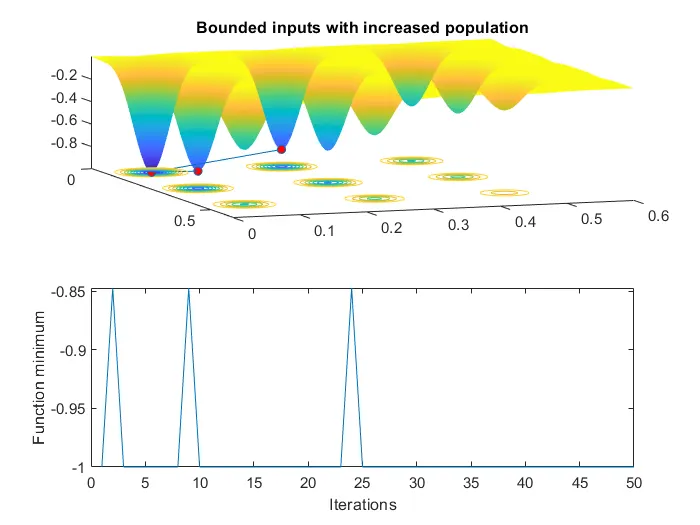
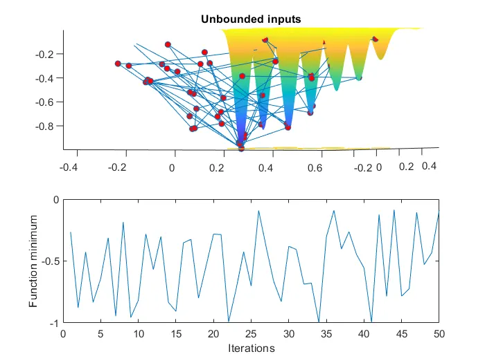
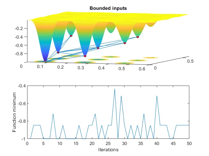
Three plots are obtained from the program;

1st plot is of study 1,

2nd plot is of study 2,

3rd plot is of study 3.

plots are attached below:

• IMAGE -1 :

• IMAGE -2 :

• IMAGE -3 :