Week 3 - Solving second order ODEs

OBJECTIVE :-

The way the pendulum moves depends on the Newtons second law. When this law is written down, we get a second order Ordinary Differential Equation that describes the position of the "ball" w.r.t time.

Similarly, there are hundreds of ODEs that describe key phenomena and if you have the ability to solve these equations then you will be able to simulate any of theses systems.

AIM :-

g = gravity in m/s2,

L = length of the pendulum in m,

m = mass of the ball in kg,

b=damping coefficient.

Write a program in Matlab\Octave that will simulate the pendulum motion, just like the one shown in the start of this challenge.

use,

L=1 metre,

m=1 kg,

b=0.05.

g=9.81 m/s2.

Simulate the motion between 0-20 sec, for angular displacement=0,angular velocity=3 rad/sec at time t=0.

EQUATION :-

PROGRAM :-

clear all
close all
clc


b=0.05;
g=9.81;
l=1;
m=1clear all
close all
clc


b=0.05;
g=9.81;
l=1;
m=0.1;

%initial condition
theta_0 = [0;5];

%time points
t_span = linespace(0,10.500);

% solve ODE
[t,results] =ode45(@(t,theta) ode_func(t,theta,b,g,l,m),t_span,theta_0);

plot(t,results(:,1))
hold on
plot(t,results(:,2))
ylabel('plot')
xlabel('time');

%initial condition
theta_0 = [0;5];

%time points
t_span = linspace (0,10,500);

% solve ODE
[t,results] =ode45(@(t,theta) ode_func(t,theta,b,g,l,m),t_span,theta_0);

plot(t,results(:,1))
hold on
plot(t,results(:,2))
ylabel('plot')
xlabel('time')

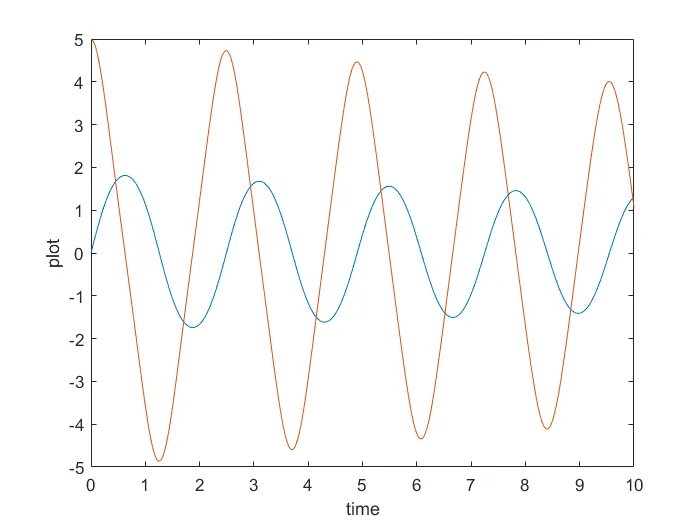
RESULTS :-

The first curve represents 'displacement'.

Tha second curve represents 'Velocity'.

Displacement starts at '0' and velocity starts at '5'.