Week 4.1 - Genetic Algorithm

Aim:

1. Write a code in MATLAB to optimize the stalagmite function and fine the global maxima of the function.
2. Clearly explain the concept of the genetic algorithm
3. Make sure that the code returns same output even if it is run several times.
4. Plot graphs for all three studies and for F maximum vs number of iterations. Title of the axes and labels is a must.

Theory:

Genetic algorithm is a method of solving problems, finding optimum solutions for both constrained and unconstrained equations. This algorithm is based on the theory of natural selection. Where the optimum solutions is found by selecting ‘children’ from the current population at random and finding the best possible solution.

Genetic algorithm uses three main types of rules at each step to create next generation from the current population:

1. Selection rule selects the individuals called parents that contribute to the population at the next generation.
2. Crossover rules combine two parents selected at random to form children in the following generation
3. Mutation rules are applied randomly to the parents while forming children

Explanation of the code:

1. Initially two variables x and y are defined taking up 150 values between 0 and 0.6 using inbuilt MATLAB command ‘linspace’
2. Two for loops are run from i=1 to the number of rows of the matrix, and a nested for loop from j=1 to number of columns of the matrix.
3. Then the stalagmite function is called in which the input from the matrix is passed.
4. The stalagmite function returns a single value ever time the for loops are run.
5. This value is stored in another matrix called ‘f’.
6. Similarly, now the stalagmite function is called again for optimization.
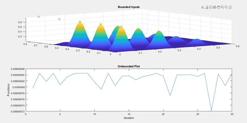
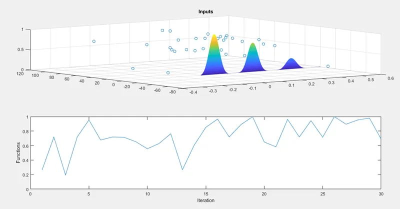
7. Then figure 1 is plotted containing the surface of the stalagmite function. Along with optimization points are plotted on the same graph, using ‘plot3()’, inbuilt function.
8. In the second part of the plot, the optimization values obtained form the stalagmite function are plotted.
9. Similarly, the stalagmite function is called again and passed for two other iterations that are bounded and unbounded.
10. User defined Stalagmite Function
    1. This function take a single value as the input and performs the function as per the equation
    2. Then returns a negative function value.

Plot 1:

Plot 2:

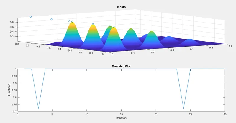
Plot3:

%Optimisation Function

clear all
close all
clc

%Defining the two variables
x=linspace(0,0.6,150);
y=linspace(0,0.6,150);

trials=30;

%Creating a 2D mesh array
[xx yy ]= meshgrid(x,y);

%Evaluating the staligmite function
for i=1 : length(xx)
    for j=1 : length(yy)
        input_vector(1)= xx(i,j);
        input_vector(2)= yy(i,j);
        f(i,j)=stalagmite(input_vector);
    end
end

tic;

for k=1: trials
    [result localval1(k)] = ga(@stalagmite, 2);
    xresult1(k)=result(1);
    yresult1(k)=result(2);
end

time1=toc;

figure(1)
subplot(2,1,1)
surf(xx, yy, -f );
shading interp
hold on
plot3(xresult1,yresult1,-localval1, 'o')
title('Inputs')
subplot(2,1,2)
plot(-localval1)
xlabel('Iteration')
ylabel('Functions')


%Study 2 Bounded plot
for p=1: trials
    [result localval2(p)] = ga(@stalagmite, 2,[],[],[],[],[0;0],[1;1]);
    xresult2(p)=result(1);
    yresult2(p)=result(2);
end

figure(3)
subplot(2,1,1)
surfc(xx, yy, -f );
shading interp
hold on
plot3(xresult2,yresult2,-localval2, 'o')
title('Inputs')
subplot(2,1,2)
plot(-localval2)
xlabel('Iteration')
ylabel('Functions')
title('Bounded Plot')


%Study 3 Unbounded

options = optimoptions('ga');
options = optimoptions(options, 'PopulationSize', 200);

for q=1: trials
    [result localval3(q)] = ga(@stalagmite, 2,[],[],[],[],[0;0],[1;1],[],[],options);
    xresult3(q)=result(1);
    yresult3(q)=result(2);
end

figure(5)
subplot(2,1,1)
surfc(xx, yy, -f );
shading interp
hold on
plot3(xresult3,yresult3,-localval3, 'o')
title('Bounded Inputs')
subplot(2,1,2)
plot(-localval3)
xlabel('Iteration')
ylabel('Functions')
title('Unbounded Plot')


[inputs, fval] = ga(@stalagmite, 2);
fout=-fval
inputs





%Stalagmite Function - User Defined

function [op2] = stalagmite(input_vector)

ip1=input_vector(1);
ip2=input_vector(2);

fx1=(sin((5.1*3.1415*ip1)+ 0.5))^6;
fy1=(sin((5.1*3.1415*ip2)+ 0.5))^6;

fx2= exp(-4*log(2)*(((ip1-0.0667)^2)/0.64));
fy2= exp(-4*log(2)*(((ip1-0.0667)^2)/0.64));

op = fx1*fy1*fx2*fy2;
op2= -(fx1*fy1*fx2*fy2);

end