Week 3 - Solving second order ODEs

Youtube link

https://www.youtube.com/watch?v=xVui5brtS4o

Screenshot of result:

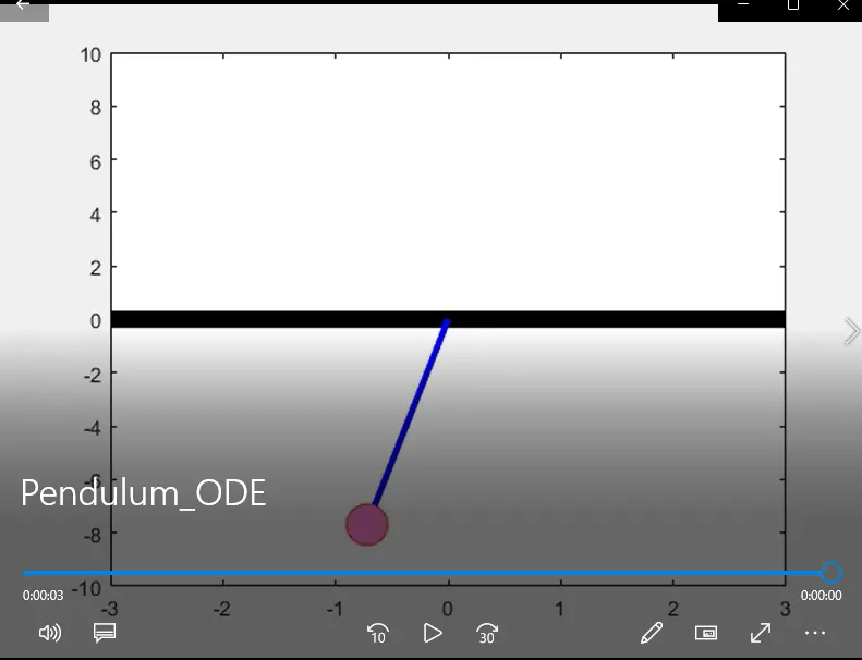
Second Order ODE

1. Defining the input variables as b , g , l and m.
2. Using function ‘linspace’ to define array called ‘tspan’ ranging from 0 to 20 seconds with 100 values in between.
3. Using inbuilt function ‘ode45’ to solve the second order ODE.
4. In ‘ode45’, a user defined function has been called which passes the input values and brakes down the equation into two simple first order ODEs.
5. Defining the coordinates of the top black line. Ranging from y=0 to 1 and in x axis ranging from -10 to 10.
6. Defining the top coordinates of the pendulum. The the length of the pendulum is taken as 1 meter.
7. Starting for loop to run from j=1 to the end of the array y, considering all the values present in the array.
8. In order to get the coordinate of the other point of the pendulum we need to get the angle first. For this creating an array called ‘phi’ which takes in the invers tan values from the matrix y.
9. Then using inbuilt function ‘rad2deg’, to convert angle in radians to degree.
10. Using trigonometry to solve the second position of the pendulum string.
11. Firstly plotting the top black line.
12. Defining the axes from x coordinates (-3 to 3) and y coordinates (-10 to 10).
13. Defining the coordinates for the ball. Taking the length of the string for visual purpose to be 7 units.
14. Plotting the string of the pendulum.
15. Plotting the ball end using function ‘markersize’, having coordinates ‘Ballx and Bally’.
16. Using inbuilt function ‘clf’ to clear the figure every time at the end of the for loop.
17. Then recording the motion in a file called ‘Pendulum_ODE.avi’.

Errors

1.

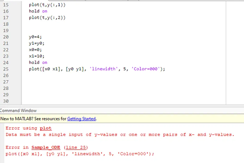
Wrong usage of function color.

2.

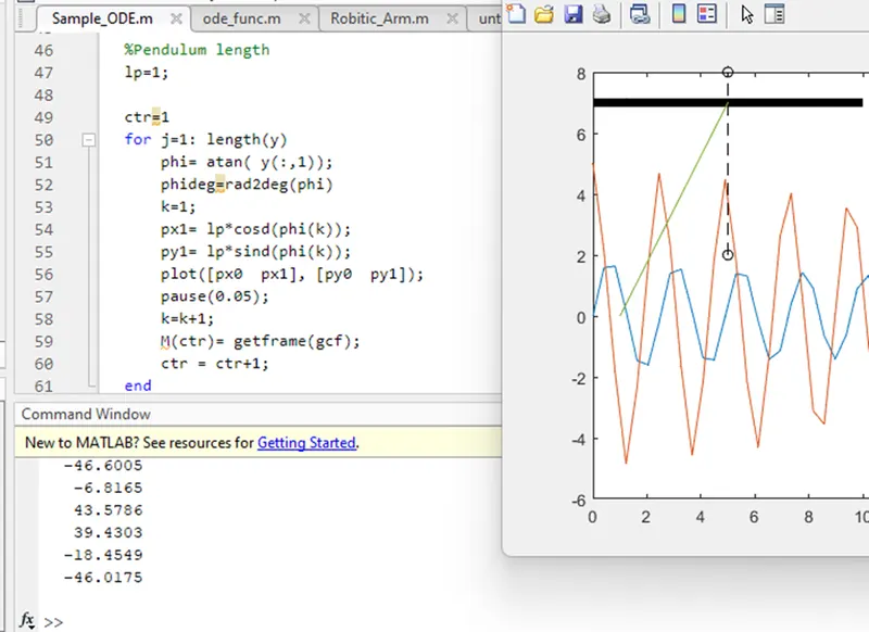
The position of the pendulum did not move. (logical error)

3.

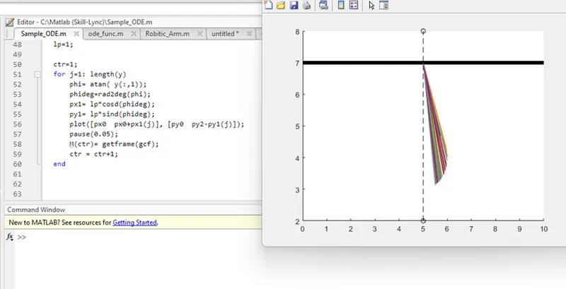
Pendulum running only on one side.

close all
clear all
clc

%Definign the initial values to solve the ODE
b=0.05;
g=9.81;
l=1;
m=1;

%defining time from 0 to 20
tspan=linspace(0,20,100);
theta0=[0;5];

%calling the user defined function to solve Pendulum equation
[t,y]= ode45(@(t,theta) ode_func (t, theta, b, m , g , l), tspan, theta0);

%Top black line coordinates
y0=0;
y1=y0;
x0=-10;
x1=10;
    
%Pendulum motion

%Pendulum top coordinates
px0=0;
py0=0;

%Pendulum length
lp=1;

ctr=1;

%for loop running from 1 to the complete length of the array y
for j=1: length(y)

    %Using trigonometry to get the angle 'phi'
    %Tan inverse inbuilt function
    phi= atan( y(:,1));
    %Converting the angel from radians to degree
    phideg=rad2deg(phi);
    %Calculating coordinate position for the other end of pendulum
    px1= lp*sind(phideg);
    py1= lp*cosd(phideg);

    figure(1)

    %Plotting the Top line
    %plot([0 0],[5 -5], '--or', 'color', [0,0,0]);
    plot([x0 x1], [y0 y1], 'linewidth', 8, 'Color',[0,0,0]);
    %Defining the  position of the axis
    axis([-3 3 -10 10]);
    
    %coordinates for the ball at the end of the string
    Ballx=px1(j);
    Bally=-7-py1(j);

    %Plotting the line
    line([px0  Ballx], [py0  Bally], 'LineWidth', 3, 'Color', 'b' );
    hold on

    %plotting the ball at the end
    plot(Ballx, Bally , 'O', 'markersize', 20, 'markerfacecolor', [1 0.5 0.8]);
    pause(0.05);
    M(ctr)= getframe(gcf);
    ctr = ctr+1;

    %clearing the figure with each run of the for loop
    clf(figure(1))
end

%Recording the motion
movie(M)
videofile = VideoWriter('Pendulum_ODE.avi', 'Uncompressed AVI');
open (videofile)
writeVideo(videofile,M)
close(videofile)






ODE User Defined function
function [dtheta_t]= ode_func (t, theta, b, m , g , l)

%Braking down the equation into smaller parts
theta1=theta(1);
theta2=theta(2);
dtheta1_t = theta2;
dtheta2_t =  -(b/m)*theta2 - (g/l)*sin(theta1);

dtheta_t = [dtheta1_t ; dtheta2_t];

end