Week 4.1 - Genetic Algorithm

>>Main Code

close all
clear all
clc

%Given x,y values 
x= linspace(0,0.6,150);
y= linspace(0,0.6,150);

%Make a 2d graph by coordinates of x,y
[xx yy] = meshgrid(x,y);

%Find input vector 
for i = 1:length(xx)
    for j =1:length(yy)
        input_vector(1)=xx(i,j);
        input_vector(2)=yy(i,j);
        f(i,j)= stalagmite(input_vector);
    end
end

%study(1)
%Area of graph is not defined
%Find maximum value with unbounded region

%Repeat order numbers
num_cases=100;

tic
 
for i=1:num_cases
    [inputs,fopt(i)]=ga(@stalagmite,2);
    xopt(i)=inputs(1);
    yopt(i)=inputs(2);
end
%GA is used to find minium values
%Inverting the equation we can get Max values
fopt=-fopt;
time_study1=toc

%Plot unbounded method results
figure(1)

%subplot(row,column,position of table)
subplot(2,1,1)  %Use to form a table
hold on
surfc(xx,yy,f)
xlabel('x-axis')
ylabel('y-axis')
%shading function controls the color shading of surface
shading interp
%plot3(x,y,z) plot coordinates in 3d space
plot3(xopt,yopt,fopt,'marker','o','markersize',5,'markerfacecolor','r')
title('Unbound method')
%figure(2)
subplot(2,1,2)
%Graph shows value of fopt at different iteration
plot(fopt)
xlabel('Iteration')
ylabel('Function maximum')
saveas(1,'GA with Unbounded method','jpg')

%study(2)
%Area of graph is defined
%Find maximum value with in bounded region
tic
for i=1:num_cases

    [inputs1,fopt1(i)]=ga(@stalagmite,2,[],[],[],[],[0,0],[0.6,0.6]);
    xopt1(i)=inputs1(1);
    yopt1(i)=inputs1(2);
end
fopt1=-fopt1;
Time_study2=toc;

figure(2)
subplot(2,1,1)
hold on
surfc(xx,yy,f)
xlabel('X-axis')
ylabel('Y-axis')
shading interp
title('Bound Method')
plot3(xopt1,yopt1,fopt1,'marker','o','markersize',5,'markerfacecolor','r')
%figure(2)
subplot(2,1,2)
plot(fopt1)
xlabel('Iterations')
ylabel('Function Maximum')
saveas(2,'GA with Bound method','png')

%study(3)
%Area of graph is defined 
%Find maximum value with bounded region,
% Optimization of options
options= optimoptions('ga');
options=optimoptions(options,'PopulationSize',500);

tic
for i=1:num_cases
    %x = ga(fun,nvars,A,b,Aeq,beq,lb,ub,nonlcon,intcon,options)
    [inputs2,fopt2(i)]=ga(@stalagmite,2,[],[],[],[],[0,0],[0.6,0.6],[],[],options)
    xopt2(i)=inputs2(1);
    yopt2(i)=inputs2(2);
end
fopt2=-fopt2;
Time_study3=toc;

figure(3)
subplot(2,1,1)
hold on
surfc(xx,yy,f)
shading interp
plot3(xopt2,yopt2,fopt2,'marker','o','markersize',5,'markerfacecolor','auto')
title('Bounded method with optimum function')
xlabel('X-axis')
ylabel('Y-axis')
%figure(2)
subplot(2,1,2)
plot(fopt2)
xlabel('Iterations')
ylabel('Function maximum')
saveas(3,'GA with optimization','png')

>> Stalagmite function code

    
function f = stalagmite(input_vector)
x=input_vector(1);
y=input_vector(2);
term1=(sin(5.1*pi*x+0.5))^6;
term2=(sin(5.1*pi*y+0.5))^6;
term3=exp(-4*log(2)*((x-0.0667)^2/0.64));
term4=exp(-4*log(2)*((y-0.0667)^2/0.64));

f = -term1*term2*term3*term4;
end

What is GA:-

-A genetic algorithm (GA) is a method for solving both constrained and unconstrained optimization problems based on a natural selection process that mimics biological evolution. The algorithm repeatedly modifies a population of individual solutions.

>> Method to find GA in Matlab

1) Unbounded Method:-

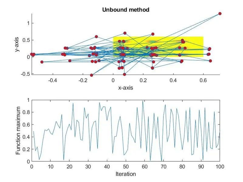
-In this method area for finding the maximum value in the Surface, is not fixed. So it can give data also from outside the region.

2) Bounded method:-

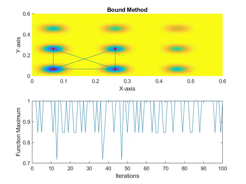
In this method Area to find maximum values is pre-determined. so we can get maximum value within the region.

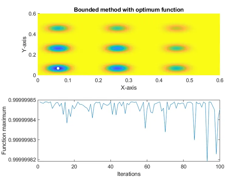
3)Bounded method with optimization (Increased 'population size')

-In this optimization of options, to get very accurate results.

>>Syntax of GA

[inputs,fval] = ga(fun,nvars,A,b,Aeq,beq,lb,ub,nonlcon,intcon,options)

>>Outputs of Coding