Week 4.1 - Genetic Algorithm

Aim: To optimize the stalagmite function & to find the global maxima of the function

Genetic algorithm:

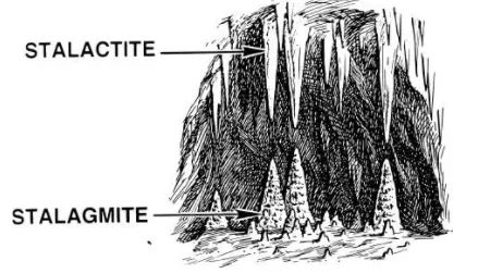
Stalactite are the structures formed from mineral deposits that hang from caves. These formations hold tightly to the ceiling & hang down. As opposed to hanging from the ceiling, Stalagmite structures are formed from the cave floor that point upward. Stalagmite & Stalactite are mathematical functions which represents shape similar to that of the stalagmite & stalactite functions.

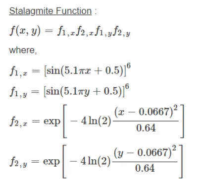
Stalagmite function:

Genetic Algorithm:

Genetic algorithm (GA) is the optimization technique used to solve non linear optimization problem. It uses concept of evolutionary biology(Darwin’s theory) to find global minima for the optimization a problem. An initial set of solutions is tested against the objective function. Subsequent generations evolve through process mentioned below:

GA done in 3 steps:

Selection: Number of individuals is selected from the population in the mating pool. Based on previously calculated fitness value, the best individual based on threshold is selected. After that we’ll end the selecting subset of the population from the pool.

Crossover: Crossover in GA generates new generation same as the natural mutation. By mutating old generation parents, the new generation offspring comes by carrying genes from both the parents. The amount of genes carried from each parent is random.

Mutation: For each offspring select some genes & change its value. Mutation prevents the solution from falling into a local minima.

Syntax:

X = ga(func, nvar)

X = ga(func, nvar) finds a local unconstrained minimum ‘x’, to the objective function,’fun’. ‘nvar’ is the number of design variables to the function ‘fun’.

Code:

First created Stalagmite function separately with the equations mentioned above.

In Genetic algorithm code first distributed X & Y axis evenly. Using meshgrid command extracted all the mating coordinates for the area. Carried out two for loops for the ‘input_vetor’ which was the calling input for the Stalagmite function. Called the function at the end. Generated the required graph using ‘surfc’ command.

As the function was giving global minima & our aim is to find global maxima modified the output variable of the Stalagmite function with the ‘–‘ sign. After this the got the global maxima value but the graph was found to be inverted 180. So, changed the surface command output to’-‘ & got the desired output.

Bounding is given in next case in order to increase accuracy. Population size increased in successive cases to reduce the bandwidth.

%Stalagmite function
function [f] = stalagmite(input_vector)

    f1x = (sin((5.1*pi).*input_vector(1) + 0.5)).^6;
    f1y = (sin((5.1*pi).*input_vector(2) + 0.5)).^6;
    f2x = exp((-4*log(2).*(input_vector(1) - 0.0667).^2/0.64));
    f2y = exp((-4*log(2).*(input_vector(2) - 0.0667).^2/0.64));

    f_x_y = f1x*f2x*f1y*f2y;
    f= -f_x_y;
end




%Defining our search space
x = linspace(0,0.6,300);
y = linspace(0,0.6,300);
limit = 30;

%Creating a 2 dimensional mesh
[xx yy] = meshgrid(x,y);

%Evaluating the Stalagmite function
for i = 1:length(xx)
    for j = 1:length(yy)
        input_vector(1) = xx(i,j);
        input_vector(2) = yy(i,j);
        f(i,j) = stalagmite(input_vector);
    end
end


tic
for i = 1:limit

    [input, fval(i)] = ga(@stalagmite,2)
    x_out(i) = input(1);
    y_out(i) = input(2);
    
end
case_time_1 = toc

figure(1)
subplot(2,1,1)
surfc(xx,yy,-f)
xlabel('X value')
ylabel('Y value')
title('Case 1 Unbounded','color','k')
shading interp
hold on;
plot3(x_out, y_out,-fval,'marker','o','markersize',6, 'markerfacecolor','r');
subplot(2,1,2)
plot(-fval);
xlabel('No of Iterarions')
ylabel('Maximum function value')


%Case 2 : Inserting Bounding Box
tic
for i  = 1:limit
    [input, fval(i)] = ga(@stalagmite,2,[],[],[],[],[0;0],[0.6;06]);
    x_out(i) = input(1);
    y_out(i) = input(2);
    
end
case_time_2 = toc
figure(2)
subplot(2,1,1)
hold on;
surfc(xx,yy,-f)
xlabel('x')
ylabel('y')
title('case 2','color','k')
shading interp
plot3(x_out,y_out,-fval,'marker','o','markersize',6,'markerfacecolor','r');
subplot(2,1,2)
plot(-fval)
xlabel('No of iterations')
ylabel('Maximum function value')




%Case 3
options = optimoptions('ga');
options = optimoptions(options,'populationsize',100)

tic
for i = 1:limit
    [input, fval(i)] = ga(@stalagmite,2,[],[],[],[],[0;0],[0.6;0.6],[],[],options);
    x_out(i) = input(1);
    y_out(i) = input(2);
    
end
case_time_3 = toc
figure(3)
subplot(2,1,1)
hold on;
surfc(xx,yy,-f)
xlabel('x')
ylabel('y')
title('case 3','color','k')
shading interp
plot3(x_out,y_out,-fval,'marker','o','markersize',6,'markerfacecolor','r');
subplot(2,1,2)
plot(-fval)
xlabel('No of iterations')
ylabel('Maximum function value')



%Case 4
options = optimoptions('ga');
options = optimoptions(options,'populationsize',300);

for i = 1:limit
    [input, fval(i)] = ga(@stalagmite,2,[],[],[],[],[0;0],[0.6;0.6],[],[],options);
    x_out(i) = input(1);
    y_out(i) = input(2);
    
end
case_time_4 = toc
figure(4)
subplot(2,1,1)
hold on;
surfc(xx,yy,-f)
xlabel('x')
ylabel('y')
title('case 4','color','k')
shading interp
plot3(x_out,y_out,-fval,'marker','o','markersize',6,'markerfacecolor','r');
subplot(2,1,2)
plot(-fval)
xlabel('No of iterations')
ylabel('Maximum function value')

Errors faced:

The min value was not getting ‘0’. As one the parenthesis in the sin bracket was missing.

After addition got the desired result.

Conclusion:

Stalagmite function run successfully to get the global minima as well as Global maxima value.