Week 4.1 - Genetic Algorithm

Aim- To write a code to optimise a stalagmite functionand find a global maximum of the function.

The concept of genetic algorithim

genetic algorithim is search based optimization technique based on the principles of genetics and natural selection, it's frequently used to find optimal or near optimal solutions to difficult problems otherwise which would take life time to solve it. It's inspired from charle's darwin of natural evolution.and charle's darwin theory is based on survival of the fittest.

it selects set of indiviuals from the population, fitness function is given to set of indiviuals based on fitness score crossover is done, and mutation is done at last for changing the gene of indiviual parent.

clear all
close all
clc

%defining the search space
x = linspace(0,0.6,150);
y = linspace(0,0.6,150);

[xx yy] = meshgrid(x,y);

num_cases = 50



%creating a 2-D dimensional array

%creating a 2-D dimensional array
for i=1:length(xx)
    for j= 1:length(yy)
        input_vector(1)= xx(i,j);
        input_vector(2)= yy(i,j);
        f(i,j)= stalagmite(input_vector);
        
    end 
end 

%statistical behaviour with unbounded inputs

for i= 1:num_cases
    [inputs, fopt(i)] = ga(@stalagmite,2);
    xopt(i) = inputs(1);
    yopt(i) = inputs(2);
end

figure(1)
subplot(2,1,1)
hold on
surfc(x, y, -f)
shading interp
plot3(xopt,yopt,-fopt,'marker','o','markersize',5,'markerfacecolor','r')
title('unbounded inputs')
subplot(2,1,2)
plot(-fopt)
xlabel('iterations')
ylabel('function maximum')


%statistical behaviour with upper and lower bounds

    

for i= 1:num_cases
    [inputs, fopt(i)] = ga(@stalagmite,2,[],[],[],[],[0;0],[1;1]);
    xopt(i) = inputs(1);
    yopt(i) = inputs(2);
end

figure(1)
subplot(2,1,1)
hold on
surfc(x, y, -f)
shading interp
plot3(xopt,yopt,-fopt,'marker','o','markersize',5,'markerfacecolor','r')
title('bounded inputs')
subplot(2,1,2)
plot(-fopt)
xlabel('iterations')
ylabel('function maximum')

%study increasing ga iteration
options= optimoptions('ga')
options= optimoptions(options,'populationsize',200)



for i= 1:num_cases
    [inputs, fopt(i)] = ga(@stalagmite,2,[],[],[],[],[0;0],[0.1;0.1]);
    xopt(i) = inputs(1);
    yopt(i) = inputs(2);
end

figure(1)
subplot(2,1,1)
hold on
surfc(x, y, -f)
shading interp
plot3(xopt,yopt,-fopt,'marker','o','markersize',5,'markerfacecolor','r')
title('bounded inputs')
subplot(2,1,2)
plot(-fopt)
xlabel('iterations')
ylabel('function maximum')

Syntax of genetic algorithim-

syntax according to matlab

x = ga(fun,nvars,A,B.Aeq.Beq,LB,UB.nonlcon,intcon,options)

fun = objective function

nvars = number of variables

A and B = subject to linear inequalities of the form A*x <=B

Aeq and Beq = subject to linear equalities of the form Aeq*x = Beq

LB = lower bound

UB = upper bound

nonlcon = non linear inequalities

intcon = integer constrained

options = helps to add contraint tolerance by increasing the population size

study1-

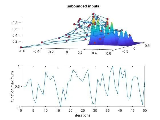
In the first study there are no lower and upper bounds defined so it's optimum value keeps changing each time the ga function is run.

study 2-

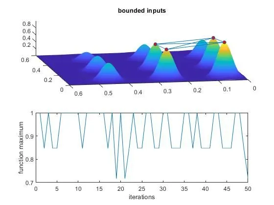
the second study lower and upper bounds are defined, so most of the optimum value lies between 1 and 0.8.

study 3-

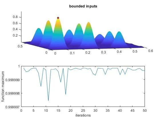
clearly we can see the global maximum lies between x value of 0-0.1 and y value of 0-0.1

so, by this we can reduce the upper and lower bounds of x and y and find the global maxima value.

step wise explanation of the code-

1)code starts with clear all,close all,clc which are the basic command before starting the code

2) then x array and y array are defined using linspace command.

3)then 2-D array is formed using meshgrid.

3)with the help of values of meshgrid, inputs are given to the stalagamite function which is defined in other window.

4) number of iterations is already defined, so the iteration are done for given number of time.

5)the other for loop is for saving inputs for stalagmite function and optimum value.

6)there are two plots are plotted one is x,y and maximum of 'f' and other plot for how f is varying with each iterations

the problem with this plot was there was no certain bounded limis.

7) And the study 2 is done with given boundedd limits.

8)but plot with study2 was there were 50 iteration possible, so now population size is increased now so that we can find much clear idea on global maxima

Errors faced while executing program-

there were no complex errors apart from the graph i was plotting was for minimum value.

steps taken to overcome the errors-

as genetic algorithim finds a minimum value, so -f will lead to find the least value which will be a maxima for us.

Online material used for research-

https://www.youtube.com/watch?v=FwPgHgbncPk

mathwork search help for understanding genetic algoithim syntax.