Week 4.1 - Genetic Algorithm

x = ga(fun,nvars,A,b) finds a local minimum x to fun, subject to the linear inequalities A*x ≤ b. ga evaluates the matrix product A*x as if x is transposed (A*x').

x = ga(fun,nvars,A,b,Aeq,beq) finds a local minimum x to fun, subject to the linear equalities Aeq*x = beq and A*x ≤ b. (Set A=[] and b=[] if no linear inequalities exist.) ga evaluates the matrix product Aeq*x as if x is transposed (Aeq*x').

x = ga(fun,nvars,A,b,Aeq,beq,lb,ub) defines a set of lower and upper bounds on the design variables, x, so that a solution is found in the range lb ≤ x ≤ ub. (Set Aeq=[] and beq=[] if no linear equalities exist.)

x = ga(fun,nvars,A,b,Aeq,beq,lb,ub,nonlcon) subjects the minimization to the constraints defined in nonlcon. The function nonlcon accepts x and returns vectors C and Ceq, representing the nonlinear inequalities and equalities respectively. ga minimizes the fun such that C(x) ≤ 0 and Ceq(x) = 0. (Set lb=[] and ub=[] if no bounds exist.)

x = ga(fun,nvars,A,b,Aeq,beq,lb,ub,nonlcon,options) minimizes with the default optimization parameters replaced by values in options. (Set nonlcon=[] if no nonlinear constraints exist.) Create options using optimoptions.

x = ga(fun,nvars,A,b,Aeq,beq,lb,ub,nonlcon,intcon) or x = ga(fun,nvars,A,b,Aeq,beq,lb,ub,nonlcon,intcon,options) requires that the variables listed in intcon take integer values.

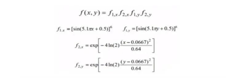
• First create a stalagmite function to split up the terms of the above equations into smaller terms
• Then use the smaller terms and combine them together using the multiplication
• Add a minus symbol and assign them to a variable

function [fxy] = stalagmite_fn(input_vector)
%defining stalagmite function
x = input_vector(1);
y = input_vector(2);
%converting the formula into simpler terms
f1x = (sin((5.1*pi*x)+0.5))^6;
f1y = (sin((5.1*pi*y)+0.5))^6;
f2x = exp(-4*log(2)*(((x-0.0667)^2)/0.64));
f2y = exp(-4*log(2)*(((y-0.0667)^2)/0.64));
%combining the terms and adding the inversion
fxy = -(f1x.*f1y.*f2x.*f2y);
end

• create another function to create a 2D array using meshgrid of x & y
• loop the 2D array elements xx,yy in the stalagmite function and get the values for i,j

function [f] = stlag(x,y)
%creating a 2D array using x & y
[xx,yy] = meshgrid(x,y);
%Looping the 2D array 
for i=1:length(xx)
    for j=1:length(yy)
        input(1) = xx(i,j);
        input(2) = yy(i,j);
        f(i,j) = stalagmite_fn(input);
    end
end
end

• Then create a program for Ga
• define a search space for 1D array using linspace
• then define a value for the limit
• call in the stalg function that has the 2D array
• Then inverse the variable of the stalag function
• Then start with the statistical studies using the ga function
• in study 1 we ll be looping the stalagmite function using ga without defining any limits or bounds
• we then use 2 subplots to plot the surface and option maxima value using plot3 and plot commands
• In the plot it is found that the values are random for global maxima due to the randomness of ga
• To avoid this we use the upper and lower bounds in study 2
• we also use tic and toc function to find out the processing time for the study.
• it is seen in plot that the randomness has been reduced to a particular set of peaks due to upper bound and lower bound values
• To even optimize the Global maxima we use options and int opt commands in study 3
• we also increase the number of iterations to 500 and now repeat the same steps and plot
• Now we see that the Global maxima is now a single peak and we get the absolute value by increasing the iterations
• But at the same time it is seen that the looping or processing time is increased in study 3
• Thus by using the UB, LB and options we get the absolute Global maximum value

clear all
close all
clc

% defining our search space by 1D array
x = linspace(0,0.6,150);
y = linspace(0,0.6,150);
num_cases = 50;
f = stlag(x,y);
F=-f
%study 1 - statistical behavior
for i = 1:num_cases
    [inputs,fopt(i)] = ga(@stalagmite_fn,2);
    xopt(i) = inputs(1);
    yopt(i) = inputs(2);
end
figure(1)
subplot(2,1,1)
hold on
surfc(x,y,f);
shading interp
plot3(xopt,yopt,fopt,'marker','o','MarkerSize',5,'markerfacecolor','r');
title('unbound Ips')
subplot(2,1,2)
plot(fopt)
xlabel('Iterations')
ylabel('fn max')
%study 2 statiscal behaviour with ub and lb
tic
for i =1:num_cases
    [inputs,fopt(i)] = ga(@stalagmite_fn,2,[],[],[],[],[0;0],[1;1]);
    xopt(i) = inputs(1);
    yopt(i) = inputs(2);
end
fopt = -fopt;
study2_time = toc;
figure(2)
subplot(2,1,1)
hold on
surfc(x,y,f)
shading interp
title('with ub and lb')
xlabel('val1')
ylabel('val2')
plot3(xopt,yopt,fopt,'marker','o','markersize',5,'MarkerFaceColor','r')
subplot(2,1,2)
plot(fopt)
xlabel('Iterations')
ylabel('fn max')
%study 3 increase ga iterations
options = optimoptions('ga')
options = optimoptions(options,'PopulationSize',500)
tic
for i = 1:num_cases
    [inputs,fopt(i)]= ga(@stalagmite_fn,2,[],[],[],[],[0;0],[1.5;1.5],[],[],options);
    xopt(i) = inputs(1);
    yopt(i) = inputs(2);
end
fopt = -fopt
study3_time = toc
figure(3)
subplot(2,1,1)
hold on
surfc(x,y,f);
shading interp
title('Inc ga itrns')
xlabel('xval')
ylabel('yval')
plot3(xopt,yopt,fopt,'marker','o','MarkerSize',5,'MarkerFaceColor','r')
subplot(2,1,2)
plot(fopt)
xlabel('itrns')
ylabel('fn max')

Observation:

It is observed that the randomness of Ga can be optimized by defining the boundaries as well as increasing the number of iterations.

Conclusion:

Thus the stalagmite function is optimized to get the Global maxima Value for the governinng equation.