Project 2 - Rankine cycle Simulator

Aim:

• To create a rankine cycle simulator using matlab
• To plot t-s snd h-s plots for given inputs

Introduction:

The Rankine cycle closely describes the process by which steam engines commonly found in thermal power generation plants harness the thermal energy of a fuel or other heat source to generate electricity.

The ability of a Rankine engine to harness energy depends on the relative temperature difference between the heat source and heat sink. The greater the differential, the more mechanical power can be efficiently extracted out of heat energy, as per Carnot cycle.The efficiency of the Rankine cycle is limited by the high heat of vaporization of the working fluid.

Four processes of Rankine cycle:

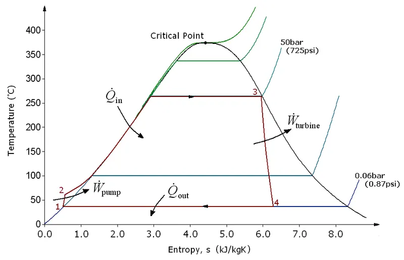
There are four processes in the Rankine cycle. The states are identified by numbers (in brown) in the T-s diagram.

• Process 1–2: The working fluid is pumped from low to high pressure. As the fluid is a liquid at this stage, the pump requires little input energy. Process 1-2 is isentropic compression.
• Process 2–3: The high-pressure liquid enters a boiler, where it is heated at constant pressure by an external heat source to become a dry saturated vapour. The input energy required can be easily calculated graphically, using an enthalpy-entropy chart (h-s chart or Mollier diagram), or numerically, using steam tables or software. Process 2-3 is constant pressure heat addition in boiler.
• Process 3–4: The dry saturated vapour expands through a turbine, generating power. This decreases the temperature and pressure of the vapour, and some condensation may occur. The output in this process can be easily calculated using the chart or tables noted above. Process 3-4 is isentropic expansion.
• Process 4–1: The wet vapour then enters a condenser, where it is condensed at a constant pressure to become a saturated liquid. Process 4-1 is constant pressure heat rejection in condenser.

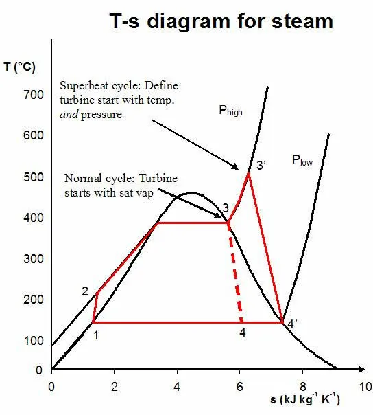
Work done on pump, per kg of water, W_P= h₂-h₁

Energy added in steam generator, q₁= h₃-h₂

Work delivered by turbine, W_T= h₃-h4

Energy rejected in the condenser, q₂= h₄-h₁

The thermal efficiency of the Rankine cycle is given by,

h= Net work done

Theory:

• Starting the program with clear all,close all and clc
• First define the processes
• Extract the satuartion temperature from Xsteam function
• Use temperature is greater than saturation temperature then extract turbine inlet pressure, Temperature at turbine inlet and turbine outlet pressure
• Use Xsteam function to extract enthalpy and entropy as function of pressure and temperature
• Evaluate the statepoints such as pressure enthalpy,entropy,temperature and the enthalpy and entropy for fluid and vapor states
• Use it to calculate the entropy and enthalpy at second state
• Then temperatures at state 3 and state 4 and also respective pressures
• Then calculate the entropy and enthalpy for the same
• Then calculate the pump work and trubine work
• After that calculate the net-work
• Calculate the heat supplied and cycle efficiency
• Finally the steam rate per second is calculated
• Then calculate the temperature at state 5 and entropy at state 5 and 6 respectively
• print the values of pressure, temperature, enthalpy and entropy for states 1,2,3 and 4 and also workdone and efficiency and steam flow rate
• write a for loop for vapour line and extract the enthalpy and entropy for liquid and vapour states
• Plot the graphs for enthalpy at liquid and vapour states vs temperature initially
• label the X and Y axis
• Then plot the enthalpy and entropy graphs for liquid and vapour states
• Then label the X and Y axis
• In the case of the temperature is less than saturation temperature then print to provide temperature greater than saturation temperature

  clear all 
  close all
  clc
  
  %Rankine cycle process 
  fprintf('1-2 Constant pressure heat transfer \n')
  fprintf('2-3 Isentropic expansion \n')
  fprintf('3-4 Constant pressure heat rejection \n')
  fprintf('4-1 Isentropic Compression \n')
  
  %Inputs
  p1 = input('Pressure at turbine inlet (in bar):');
  t1 = input('Temperature at turbine Inlet (in Degree Celcius):');
  p2 = input('Pressure at turbine outlet/Condenser Inlet pressure (in bar):');
  
  %Input condtions
  t = XSteam('Tsat_p',p1);
  if t1>=t
      h1 = XSteam('h_pT',p1,t1);
      s1 = XSteam('s_pT',p1,t1);
      %Evaluating State points
      p4 = p1;
      p3 = p2;
      h3 = XSteam('hL_p',p3);
      s3 = XSteam('sL_p',p3);
      t3 = XSteam('Tsat_p',p3);
      s2 = s1;
      t2 = t3;
      sf2 = XSteam('sL_p',p2);
      sg2 = XSteam('sV_p',p2);
      x2 = (s2-sf2)/(sg2-sf2);
      hf2 = XSteam('hL_p',p2);
      hg2 = XSteam('hV_p',p2);
      h2 = hf2 + x2*(hg2-hf2);
      s4 = s3;
      h4 = XSteam('h_ps',p4,s4);
      cp4 = XSteam('Cp_ps',p4,s4);
      cv4 = XSteam('Cv_ps',p4,s4);
      g4 = cp4/cv4;
      o = (g4-1)/g4;
      t4 = t3*((p4/p3)^o);
  
      %Turbine & Pump Work
      wt = h1 - h2;
      wp = h4 - h3;
      %net work
      wnet = wt - wp;
      %heat supplied
      qs = h1 - h4;
      %Efficiency
      n_per = (wnet/qs)*100;
      %rate fo steam per second
      stm_rate = 3600/(wt - wp);
  
      %process 4-1 the expression dH = Cp*dT
      t5 = XSteam('Tsat_p',p1);
      s5 = XSteam('sL_p',p1);
      s6 = XSteam('sV_p',p1);
  
      %output
      fprintf('\n \t RESULT \n')
      fprintf('state point 1:\n P1 is :%4.2f Bar \n T1 is :%4.2f Degree Celsius \n H1 is :%4.2f kJ/kg \n S1 is :%4.2f kJ/kgk \n \n',p1,t1,h1,s1)
      fprintf('state point 1:\n P2 is :%4.2f Bar \n T2 is :%4.2f Degree Celsius \n H2 is :%4.2f kJ/kg \n S2 is :%4.2f kJ/kgk \n \n',p2,t2,h2,s2)
      fprintf('state point 1:\n P3 is :%4.2f Bar \n T3 is :%4.2f Degree Celsius \n H3 is :%4.2f kJ/kg \n S3 is :%4.2f kJ/kgk \n \n',p3,t3,h3,s3)
      fprintf('state point 1:\n P4 is :%4.2f Bar \n T4 is :%4.2f Degree Celsius \n H4 is :%4.2f kJ/kg \n S4 is :%4.2f kJ/kgk \n \n',p4,t4,h4,s4)
      fprintf('Wt is :%4.2f kJ/kg \n Wp is :%4.2f kJ/kg \n Wnet is :%4.2f kJ/kg \n Ntherm is :%4.2f percent \n S.S.C is :%4.2f kg/kWh', wt,wp,wnet,n_per,stm_rate)
  
      %Vapour line
      temp = linspace(1,400,100);
      for i = 1:length(temp)
          ent_l(i) = XSteam('sL_T',temp(i));
          ent_v(i) = XSteam('sV_T',temp(i));
          enth_l(i) = XSteam('hL_T',temp(i));
          enth_v(i) = XSteam('hV_T',temp(i));
      end
  
      % Plot
      subplot(1,2,1)
      plot([s1 s2 s3 s4 s5 s6 s1],[t1 t2 t3 t4 t5 t5 t1],'Color','k','LineWidth',2,'Marker','*','MarkerSize',2,'MarkerFaceColor','r','MarkerEdgeColor','r')
      hold on
      plot(ent_l,temp,'Color','b')
      plot(ent_v,temp,'Color','b')
      axis([0 10 0 600])
      text(s1,t1,'1','FontSize',15)
      text(s2,t2,'2','FontSize',15)
      text(s3,t3,'3','FontSize',15,'HorizontalAlignment','right')
      text(s4,t4,'4','FontSize',15,'HorizontalAlignment','right')
      xlabel('Entropy')
      ylabel('Temperature')
      subplot(1,2,2)
      plot([s1 s2 s3 s4 s1],[h1 h2 h3 h4 h1],'Color','k','LineWidth',2,'Marker','*','MarkerSize',2,'MarkerFaceColor','r','MarkerEdgeColor','r')
      axis([0 10 50 3500])
      hold on
      plot(ent_v,enth_v,'Color','b')
      plot(ent_l,enth_l,'Color','b')
      text(s1,h1,'1','FontSize',15)
      text(s2,h2,'2','FontSize',15)
      text(s3,h3,'3','FontSize',15,'HorizontalAlignment','right','VerticalAlignment','top')
      text(s4,h4,'4','FontSize',15,'HorizontalAlignment','right','VerticalAlignment','bottom')
      xlabel('Entropy')
      ylabel('Enthalpy')
  
  else
      fprintf('Please enter temperature greater than or equal to saturation temperature')
  end
  ​

Conclusion:

Thus the rankine cycle is simulated successfully using matlab and the efficiency , workdone and plots are shown respectively