Week 4.1 - Genetic Algorithm

AIM: Write a code in MATLAB to optimise the stalagmite function and find the global maxima of the function.

OBJECTIVE:

• To explain the concept of genetic algorithm and also explain the syntax for ga in MATLAB.
• To Make sure that the code gives the same output, even if it is made to run several times.

EXPLANATION:

Genetic algorithm is a method which is taken from Charles Darwin's theory of evolution, which is used to solve both constrained and unconstraind optimization problerms . Genetic algoritm is one of the optimiazation method used in Matlab. this algorithm is based on genetic and Natural selection.

Optimization is the process of taking a set of inputs and trying to get the best output values in order to achivie a best optimal solution from the inputes given

Basically if there is need to design a rotating shaft, as a designer one should be aware of the parameters to be considered while designing a shaft, such as length, inner diameter, outer daimeter, bending stress , RPM and shear stress. all this desigen parameters as considerd as the inputes. using Ga method this inputs are crossed over several times to produce a best set of output values or best set of design parameters.

CODE 1:

clear all
close all
clc
%inputes 
x=linspace(0,0.6,150);
y=linspace(0,0.6,150);
num_cases=15;
%meshing 
[xx, yy]=meshgrid(x,y);
 
% assingint the inputes to the funtion
for i=1:length(x)
    for j=1:length(y)
        z(i,j)=stalagmite([xx(i,j),yy(i,j)]);
    end
end

%case-1
rng default
for i=1:num_cases
    [inputes,fopt(i)]=ga(@stalagmite,2);
    xopt(i)=inputes(1);
    yopt(i)=inputes(2);
end

%plotting 
figure(1)
subplot(2,1,1)
hold on
surfc(x,y,z);
shading interp
title('unbounded inputes')
plot3(xopt,yopt,fopt,"marker","o","MarkerSize",5,"MarkerFaceColor","r")
subplot(2,1,2)
plot(fopt)
xlabel('itirations')
ylabel('function minima')

%study-2 whit upper and lower bounds
rng default
for i=1:num_cases
    [inputes,fopt(i)]=ga(@stalagmite,2,[],[],[],[],[0 0],[0.6 0.6]);
    xopt(i)=inputes(1);
    yopt(i)=inputes(2);
end

%ploting
figure(2)
subplot(2,1,1)
hold on
surfc(x,y,z);
shading interp
plot3(xopt,yopt,fopt,"marker","o","MarkerSize",5,"MarkerFaceColor","r")
title('bounded inputes')
subplot(2,1,2)
plot(fopt)
xlabel('itirations')
ylabel('function minima')


% chaninging the population size to 170
options=optimoptions("ga");
options=optimoptions(options,"PopulationSize",170);

rng default
for i=1:num_cases
    [inputes,fopt(i)]=ga(@stalagmite,2,[],[],[],[],[0 0],[0.6 0.6],[],[],options);
    xopt(i)=inputes(1);
    yopt(i)=inputes(2);
    inputes
end
%ploting
figure(3)
subplot(2,1,1)
hold on
surfc(x,y,z);
shading interp
plot3(xopt,yopt,fopt,"marker","o","MarkerSize",5,"MarkerFaceColor","r")
title('bounded inputes')
subplot(2,1,2)
plot(fopt)
xlabel('itirations')
ylabel('function minima')

Line 6-8:

x=linspace(0,0.6,150); -assinging the inputs values using linspace command
y=linspace(0,0.6,150);
num_cases=15;

Line 10:

[xx, yy]=meshgrid(x,y); -meshing the values of x and y using meshgrid command

Line 13-17:

for i=1:length(x) -assigning the input values to the stalagmite function using nested loop
for j=1:length(y)
z(i,j)=stalagmite([xx(i,j),yy(i,j)]);
end
end

Line 21-25:

for i=1:num_cases -using for loop to itirate the ga for the number of cases times
[inputes,fopt(i)]=ga(@stalagmite,2);
xopt(i)=inputes(1);

yopt(i)=inputes(2);
end

ga syntax -
[inputes,funtion_values]=ga(@funtion_name,no.of variables)

The inputs and the funtion_values as stored in a variable and then Ga operate is used and the funtion is called using @funtion_name and the nunber of variables used is given.

Line 43:

[inputes,fopt(i)]=ga(@stalagmite,2,[],[],[],[],[0 0],[0.6 0.6]);

ga syntax-

[inputes,funtion_values]=ga(@funtion_name,no.of variables,A,B,Aeq,Beq,lowerbound,upper bound)

Lower bound and upper bound values are assigned to determine the global maxima in that particular region of the surf plot

and rest other values are left blank

Line 63-64:

options=optimoptions("ga"); -changing the size of population from 50 to 170 using optimoptions
options=optimoptions(options,"PopulationSize",170); -command

Line 68:

[inputes,fopt(i)]=ga(@stalagmite,2,[],[],[],[],[0 0],[0.6 0.6],[],[],options);

ga syntax-

[inputes,funtion_values]=ga(@funtion_name,no.ofvariables,A,B,Aeq,Beq,lowerbound,upperbound,nonlinear contrans,integer constrains,options)

When a default set value is changed using optimoptions command, options is mentioned insied the ga syntax

CODE 2:

%declaring a funtion
function z=stalagmite(x,y)
%foumulas
x1=(sin(5.1*pi*x(1)+0.5))^6;
x2=exp(-4*log(2)*(((x(2)-0.0667)^2)/0.64));
y1=(sin((5.1*pi*x(2))+0.5))^6;
y2=exp(-4*log(2)*(((x(1)-0.0667)^2)/0.64));

z=-1*x1*x2*y1*y2;

end

Line 2:

function z=stalagmite(x,y) -creating a funtion witha funtion name stalagmite and giving the input and output variables

Line 4-7:

x1=(sin(5.1*pi*x(1)+0.5))^6; -formulas to purform a stalagmite funtion
x2=exp(-4*log(2)*(((x(2)-0.0667)^2)/0.64));
y1=(sin((5.1*pi*x(2))+0.5))^6;
y2=exp(-4*log(2)*(((x(1)-0.0667)^2)/0.64));

Line 9:

z=-1*x1*x2*y1*y2; -output for the salagmite funtion

OUTPUT:

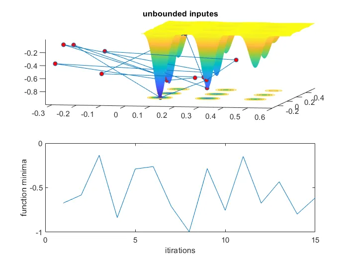
Fig(1) unbounded inputes

In the fig(1) there are 25 points represented using marker which respresent all point from the inputs.From this grap the exact location of the global maxima can not be found

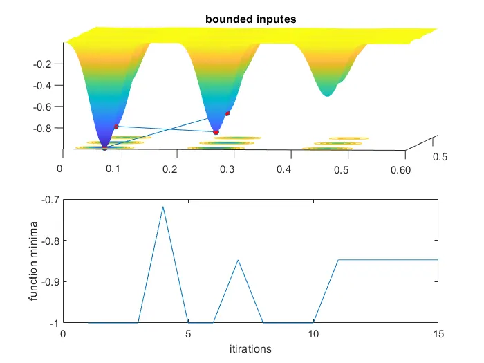
Fig(2) bounded inputes

From fig(1) its known that the peak lise between 0.6 to 0.6 , after asigning the bound values to that particular rage it's been showing that the global maxima will lise between this 4 pointes

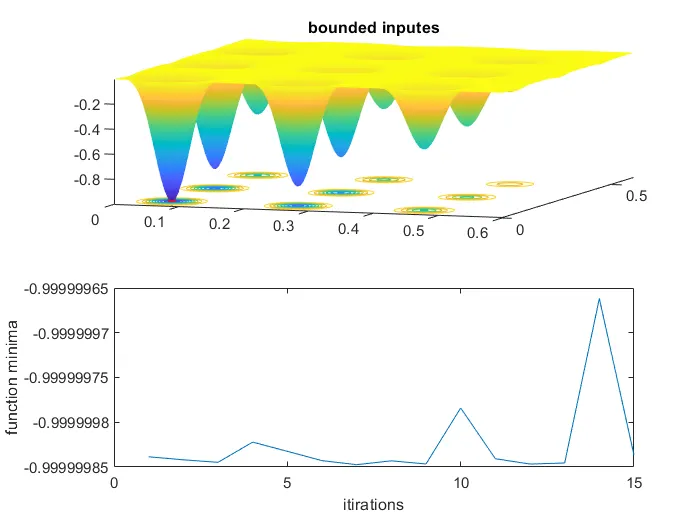
Fig(3) plot after incresing the population size

In case stude-3 once the population size is increased the globale maxima point is pointed out in the graph

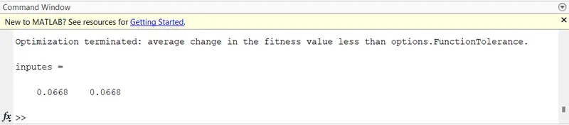
Fig(4) best optimization output value

Fig(4) shows the output for the exact location of the globle maxima and the best optimal value for the salegmite funtion

CONCLUTION:

• Using Ga the global maxima is obtained to be at 0.0668 and 0.0668
• By increasing the number of iterations or the population size optimal values can be optianed