Week 2- 2R Robotic Arm Challenge

AIM: To Write a program in Matlab to simulate the forward kinematics of a 2R Robotic Arm

• Create an animation file of the plot.

OBLECTIVE:

• To find the starting point and ending points of the 2 links of the arm
• varying the angles of the two links and determining there end-effect for different angle or θ values of the respective arm`
• To develop an animation of the plot optained for different angles or different θ values

EXPLANATION:

Consider a 2R Robotic Arm as show in the fig(1.1), the possible position of the robot arm or the end-effector of the given Arm is optained from the known value of the angular difference or θ of the respective arms of the robot. This penomenon is known as Forward kinamatics, in other words it is refferd as the use of kanamatic equation to determine the possible position of the two links with respect to there angular difference or θ. This penomenon is used to test the working and the movements of the particular robot which in turn determines the working space of the robot.

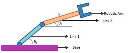
Fig(1.1) 2R ROBOTIC ARM

PROCEDURE:

STEP 1: Determine the starting point and the ending point of the link 1

• Let us consider the lenght of the link 1 is L1 as shown in the fig (1.1)
• Let us consider the starting points of link 1 as [x ,y]. As the starting point of the link 1 is at the base ,the value of [x,y] can be considered as [0,0].
• Let us consider the end point of the link 1 as [x1 ,y1]. As the link one as an angle θ1 with respect to the x-axis, the value of x1 and y1 can be optianed from the kinamatic equations.

x1=L1*cos(θ1)

y1=L1*sin(θ1) .........eq(1)

STEP 2: Determine the starting point and the ending point of the link 2

• Let us consider the lenght of the link 2 is L2 as shown in the fig (1.1)
• From fig(1.1) the starting point of the like 2 and the ending point of the link 1 are same,therefore starting point of link 2 is [x1 ,y1]
• Let us consider the end point of the link 2 as [x2 ,y2]. As the link two as an angle θ2 with respect to the x-axis, the value of x2 and y2 can be optianed from the kinamatic equations.

  x2=x1+L2*cos(θ2)

  y2=y1+L2*sin(θ2) .........eq(2)

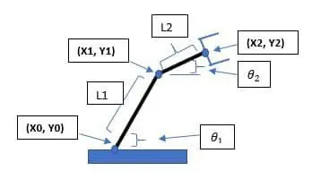
Fig (1.2) representation of the starting and ending points of the 2R robotic Arm

Lets consider,

L1=1

L2=0.5

θ1 and θ2 varying from 0 to 90 degrees.

CODE:

clear all
close all
clc
%assinging the inut values
l1=1;
l2=0.5;
%varyeing the theta value from 0-90
theta1=linspace(0,90,10);
theta2=linspace(0,90,10);
ct=1;
%creat a loop 
for i=1:length(theta1)
    THETA1=theta1(i);
    for j=1:length(theta2)
        THETA2=theta2(j);
        %coordinates
        x=0;
        y=0;
         
        x1=l1*cosd(THETA1);
        y1=l1*sind(THETA1);

        x2=x1+l2*cosd(THETA2);
        y2=y1+l2*sind(THETA2);

        plot([x x1],[y y1],[x1 x2],[y1 y2],'LineWidth',4)
        axis([-0.1 1.5 0 1.5]);
        title('simulation of forward kinematics of a 2R Robotic Arm');
        xlabel('x-axis');
        ylabel('y-axis');
       pause(0.003)
       %combining all the frames
       M(ct)=getframe(gcf);
       ct=ct+1;
  
    end
end
%creating animation
movie(M)
videofile=VideoWriter('kamanamatics_plot.avi','uncompressed AVI');
open(videofile)
writeVideo(videofile,M)
close(videofile)

Fig 1 code for forward kinematics of a 2R Robotic Arm

Line 5-6:

l1=1;

l2=0.5; -assinging the lenght of link1(l1) and link2(l2)

Line 8-9:

theta1=linspace(0,90,10);

theta2=linspace(0,90,10); -varying theta1 (θ1) and theta2 (θ2) values from 0-90 in ten equal positions using linespace command

Line 10:ct=1; -assinging variable ct with initial value one

Line 12:for i=1:length(theta1) -creating a loop of i from 1 - the length of theta1

Line 13:THETA1=theta1(i); -copying all the values of theta1 to THETA1 variable from the loop

Line 14:for j=1:length(theta2) -creating a loop of j from 1 - the length of theta1

Line 15:THETA2=theta2(j); -copying all the values of theta2 to THETA2 variable from the loop

Line 17-24:

x=0;
y=0;

x1=l1*cosd(THETA1); -assingning the values for all coordinates as mentioned in step 1 and step 2
y1=l1*sind(THETA1);

x2=x1+l2*cosd(THETA2);
y2=y1+l2*sind(THETA2);

Line 26: plot([x x1],[y y1],[x1 x2],[y1 y2],'LineWidth',4) -ploting command

Line 31: pause(0.003) -adjesting the speed of the animation

Line 33:M(ct)=getframe(gcf); -storying all the frames in a arrya M

Line 34:ct=ct+1; -incrementing ct

Line 39:movie(M) -using movie command to join all the frames in array M

Line 40:videofile=VideoWriter('kamanamatics_plot.avi','uncompressed AVI'); - creating a videofile and storing the video in .avi extention

Line 41:open(videofile) -opening the video file

Line 42:writeVideo(videofile,M) -writing video using video file and all the frames in array M

Line 43:close(videofile) -closeing the video file

OUT PUT:

Video Link:- https://youtu.be/s-IfYq8reM4

The above given video show the simulation of forward kinematics of a 2R Robotic Arm,it shows the different angle made by link1 with respect to the different angles made by link2. For one angle made by link1,links2 makes 10 different positions .

CONCLUTION:

• simulation of forward kinematics of a 2R Robotic Arm was optained from Matlad.
• The total work space of the robotic arm was determined.