Week 4.1 - Genetic Algorithm

Aim:

To write a code in matlab for stalagmite function and to find the global maxima of the function.

Code:

code for stalagmite main and global maxima:

clear all
close all
clc

%defining our search space
x=linspace(0,0.6,150);
y=linspace(0,0.6,150);
n_numb=50;

%creating a 2 dimesional mesh 
[xx, yy]=meshgrid(x,y);
    
%evaluating the stalagmite func
for i=1:length(xx);
    for j=1:length(yy);
        input_vector(1)=xx(i,j);
        input_vector(2)=yy(i,j);
        f(i,j)=stalagmite(input_vector);
    end
end

f=-f
figure(1)
surfc(xx,yy,f)
xlabel('x value')
ylabel('y vallue')

shading interp

% [x,fva1]=ga(@stalagmite,2);

%study 1-statistical behaviour
tic
for i=1:n_numb
    [inputs,f_o(i)]=ga(@stalagmite,2);
    x_o(i)=inputs(1);
    y_o(i)=inputs(2);
end

study_time_1=toc

figure(2)
subplot(2,1,1)
hold on
surfc(xx,yy,f)
shading interp
title('study 1 unbounded values')
plot3(x_o,y_o,-f_o,'marker','o','color','r')
subplot(2,1,2)
plot(f_o)
xlabel('Iterations')
ylabel('F maximum')

%study 2-statistical behaviour with upper and lower bonds
tic
for i=1:n_numb
    [inputs,f_o(i)]=ga(@stalagmite,2,[],[],[],[],[0;0],[0.6;0.6]);
    x_o(i)=inputs(1);
    y_o(i)=inputs(2);
end

study_time_2=toc

figure(3)
subplot(2,1,1)
hold on
surfc(xx,yy,f)
shading interp
title('study 2 bounded values')
plot3(x_o,y_o,-f_o,'marker','o','color','r')
subplot(2,1,2)
plot(f_o)
xlabel('Iterations')
ylabel('F maximum')

%study 3-increased populations

options=optimoptions('ga')
options=optimoptions(options,'populationsize',170)

tic
for i=1:n_numb
    [inputs,f_o(i)]=ga(@stalagmite,2,[],[],[],[],[0;0],[0.6;0.6],[],[],options);
    x_o(i)=inputs(1);
    y_o(i)=inputs(2);
end

study_time_3=toc

figure(4)
subplot(2,1,1)
hold on
surfc(xx,yy,f)
shading interp
title('study 3 increased populations')
plot3(x_o,y_o,-f_o,'marker','o','color','r')
subplot(2,1,2)
plot(f_o)
xlabel('Iterations')
ylabel('F maximum')

code for stalagmite:

function s= stalagmite(input_vector)
x=input_vector(1);
y=input_vector(2);
f1=(sin(5.1*pi*x+0.5))^6;
f2=exp(-4*log(2)*((x-0.0667)^2/0.64));
f3=(sin(5.1*pi*y+0.5))^6;
f4=exp(-4*log(2)*((y-0.0667)^2/0.64));
s=-(f1*f2*f3*f4);
end

Code explanation:

The code for stalagmite function is written first by the bassis of the formula f(x,y)=-(f1x, f2x, f1y, f2y) where f1x=[sin(5.1*pix+.5)]⁶, f1y=sin(5.1*piy+.5)]⁶, f2x=exp[-4 ln(2)((x-.0667)²/0.64)], f2y=exp[-4 ln(2)((y-.0667)²/0.64)], with the function name as stalagmite(input_vector), the input x&y are given the values of input_vector 1&2 respectivily. The minus sign it to make the genetic algorithm(ga) to find the global maxima values.

In the main code genetic algorithm(ga) is used to find the global maxima values in the stalagmite output.

First the input for the search space is assinged to x&y from 0 to 0.6 with an interval of 150 values using linspace to create 1dimensional arrays, and the number of iterations to be done is also cotted in it, then meshgrid command is used to create the 2dimensional mesh.

Then the stalagmite function is called in a for loop having i&j values with length xx & yy.

To plot this values in 3d form surfc command is used with the values xx, yy and f, and to make the surface look smooth shading interp command is used.

Then a for loop is added with limit 1 to the number of iterations that is 50, then the ga is called with the syntax @function, variable is used to call the stalagmite function which contains 2 variables, and the output values of stalagmite is stored in inputs and f_o which is the optimum value. The values in the inputs are stored in x_o and y_o containing inputs 1&2 respectivily.

As the ga function command doesn't always gives the perfect values at the first or single try, so for loop is used for a n number of times so that we can get some accurate values.

To calculate the time taking a clock timer is added using tic and toc command.

To plot the study graph and fmax vs iteration graph in a single figure we use subplot(2,1,1)&(2,1,2) in the first subplot 3d surface is plotted along with the trace of x_o, y_o, and optimum value f_o in the 2nd subplot the optimum value is plotted which is the fmax vs iteration graph.

Since the ga searches also in the outside of the boundary value we uses a 2nd study to limit the boundary with upper and lower bond values as [0;0] and [0.6;0.6], with the same procedure as the first study with adding the lower and upper bond in the for loop in ga syntax and plotted.

To get more accurate value a 3rd study is included where the population is further increased to make more divisions. As the ga takes the default value which is 50, so for two inputs x&y it takes the poplation value as 100, to change that we have to optimize the solver with the options optimotions syntax, there the solver name and the name in which the values should be changed is entered with the increased value.

The same procedure is followed here by changeing the ga syntax to ga(fun,nvars,A,b,[],[],lb,ub,nonlcon,IntCon,options) and giving the value for lower and upper bonds and for options, other all left as empty array ([]), and plotted.

Output/results:

study_time_1=

4.5890

study_time_2=

6.9182

study_time_3=

14.5391

Graphs:

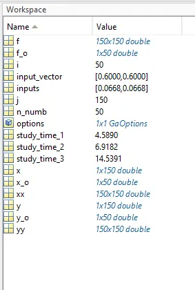
outputs in workspace

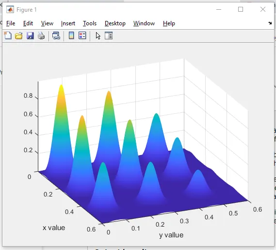
stalagmite graph

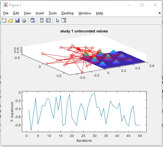
study 1 unbonded

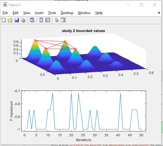
study 2 bonded

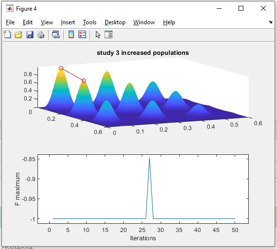
study 3 increases populations