Week 4.1 - Genetic Algorithm
AIM:
To optimize the Stalagmite function and to find Global Maxima of the function using Genitic Algorithm in MATLAB Programimng.
OBJECTIVE:
1.The objective of this report is to optimize the Stalagmite Function by coding the program with help of Gentic Algorithm using MATLAB.
2.To explain the concept of Genetic Algorithm and also explain the syntax of "ga" in MATLAB.
INTRODUCTION AND THEORY:
STALAGMITE:
A Stalagmite is a type of rock formation that rises from the floor of a cave due to the accumalation of the material deposited on the floor from celing drippings. Stalagmites are typically composed of calcium carbonate and it may consist of lava,mud,peat,pitch,sand,sinter.
Since our function gives the shape of stalagmite it is named as a Stalagmite function. It is the mathamatical model that helps us to generate minimas and maximas. It is 3D function and is designate to generate local maximas.
GENETIC ALGORITHM:
A Genetic Algorithm is a search that is based the Theory of natural evolution. This algorithm reflects the process of natural selection where the fittest indvidual is selected for reproduction in order to produce offspring of the next generation.In other words,The genetic algorithm is a method for solving both constrained and unconstrained optimization problems that is based on natural selection, the process that drives biological evolution. The genetic algorithm repeatedly modifies a population of individual solutions.
In computer science, a genetic algorithm are commonly used to generate high quality solutions to optimation and search problems by relying on biological inspired operators. The genetic algorithm can be applied to solve a variety of optimization problems that are not well suited for standard optimization problems that are not well suited for standard optization algorith including problems in which the objective function is discontinuous,non-differentiable stachastic ot highly nonlinear.It is genrealy uses of three main types of rules.They are
At each step to create the next generation from the current population:
1.SELECTION RULES:
It selects the individuals called parents that contribute to the populations at the next generation.
2.CROSSOVER RULES:
This combine two parents to form children for the next generations.
3.MUTATION RULES:
It apply random changes to individual parents to form children.
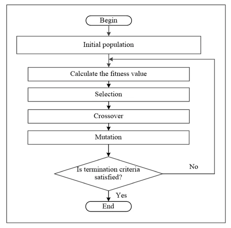
The Algorithm performs as follows:
1.It begins by crating a ramdom intialpopulations.
2.Then it scales the raw fitness scores to convert them into a more usable range of values.These scaled values are called expection values.
3.Then it selects members called parents based on thier expectations.
4.Along individuals that have high fitness value some of the individuals in the current population that have lower fitness are chosen as elite.These elite individuals are passed to the next populations. Also it produce children by making random changes to single parents-mutuation-or by combing the vector entries of a pair of parents crossover.
5.It then replaces the current population with the children to form the next generation.
6.Then it scores each member of the current populations by computing its fitness value.
7.These values are called raw fitness scores then the algorithm stops when one of the stoping criteria is meet.
FOMULA:
f(x,y) = f1,x f2,x f1,y f2,y
f1,x = [sin(5.1`pi`x + 0.5)]^6
f1,y = [sin (5.1`pi`y+ 0.5)]^6
f2,x = exp[-4ln(2)(x-0.0667)^2/0.64]
f2,y = exp[-4ln(2)(x-0.0667)^2/0.64]
The above formula are used in the stalagmite function to plot the graph in the main function in MATLAB.
FUNCTION PROGRAM:
function [f] = stalagmite(inputs)
f1x = (sin(5.1*pi*inputs(1)+0.5)).^6;
f1y = (sin(5.1*pi*inputs(2)+0.5)).^6;
f2x = exp(-4*log(2)*(((inputs(1)-0.0667)^2/(0.64))));
f2y = exp(-4*log(2)*(((inputs(2)-0.0667)^2/(0.64))));
f = -(f1x*f1y*f2x*f2y);
end
CODE EXPLANATION:
1.We creating an user defined function Stalagmite.
2.The formula to do this formual is program get defined.
3.While using the function at the end as we are using the negative(-) sign.
4.So that the plot will be reversed as we have to find the maxima of the given function using ga.
PROGRAM:
clear all
close all
clc


x = linspace(0,0.6,150);
y = linspace(0,0.6,150);
num_cases = 50;

%creating a2D meshgrid
[xx, yy] = meshgrid(x,y);

%Evaluate the stalagmite function
for i = 1:length(y)
    for j = 1:length(x)
        inputs(1) = xx(i,j);
        inputs(2) = yy(i,j);
        z(i,j) = stalagmite(inputs);
    end
end
surfc(xx,yy,-z)

% study 1 un bounded statistical behaviour
tic
for i = 1:num_cases
    [inputs, fopt(i)] = ga(@stalagmite, 2);
    xopt(i) = inputs(1);
    yopt(i) = inputs(2);
end
study1_time = toc;

figure(1)
subplot(2,1,1)
hold on
surfc(x ,y, -z)
xlabel('x-values')
ylabel('y-values')
zlabel('Function Values')
shading interp
plot3(xopt,yopt,-fopt,'marker','o','markersize',5,'MarkerFaceColor','r')
title('Unbounded Stastical Behaviour')
subplot(2,1,2)
plot(-fopt)
xlabel('Iterations')
ylabel('Function Maximum')


%study 2 statistical behaviour with upper and lower bounds
tic
for i = 1:num_cases
    [inputs, fopt(i)] = ga(@stalagmite, 2,[],[],[],[],[0;0],[1;1]);
    xopt(i) = inputs(1);
    yopt(i) = inputs(2);
end
study2_time = toc;

figure(2)

subplot(2,1,1)
hold on
surfc(x,y,-z)
xlabel('x-values')
ylabel('y-values')
zlabel('Function Values')
shading interp
plot3(xopt,yopt,-fopt,'marker','o','markersize',5,'MarkerFaceColor','r')
title('Bounded Stastical Behaviour')
subplot(2,1,2)
plot(-fopt)
xlabel('Iterations')
ylabel('Function Maximum')

 % study 3 increasing GA iterations
options = optimoptions('ga');
options = optimoptions(options,'PopulationSize',170);

tic
for i = 1:num_cases
    [inputs, fopt(i)] = ga(@stalagmite,2,[],[],[],[],[0;0],[1;1],[],options);
    xopt(i) = inputs(1);
    yopt(i) = inputs(2);
end
study3_time = toc;

figure(3)
subplot(2,1,1)
hold on
surfc(x,y,-z)
xlabel('x-values')
ylabel('y-values')
zlabel('Function Values')
shading interp
plot3(xopt,yopt,-fopt,'marker','o','markersize',5,'MarkerFaceColor','r')
title('Bounded Stastical Behaviour With Modified Population Size')
subplot(2,1,2)
plot(-fopt)
xlabel('Iterations')
ylabel('Function Maximum')

Total_time = study1_time + study2_time + study3_time;

fprintf('n The results are below : ')
fprintf('nn study 1 : unbounded statical behaviour')
fprintf('nn The time taken for the study 1 is : %f', study1_time)
fprintf('n the coordinates of x & y for the global maxima of the function are : %f,%f',inputs(1),inputs(2))
fprintf('nn the global maxima of the function is : %f',-(mean(fopt)))

fprintf('nn study 2 : unbounded statical behaviour')
fprintf('nn The time taken for the study 2 is : %f', study2_time)
fprintf('n the coordinates of x & y for the global maxima of the function are : %f,%f',inputs(1),inputs(2))
fprintf('nn the global maxima of the function is : %f',-(mean(fopt)))

fprintf('nn study 3 : unbounded statical behaviour')
fprintf('nn The time taken for the study 3 is : %f', study3_time)
fprintf('n the coordinates of x & y for the global maxima of the function are : %f,%f',inputs(1),inputs(2))
fprintf('nn the global maxima of the function is : %f',-(mean(fopt)))
PROGRAM EXPLANATION:
1.Starting the procedure with clc commands.
2.Linspace command is used to define x and y with elements of 150 between 0 and 0.6 including the bounds.
3.The num_cases is set which will be used as counter for iteration to 50.
4.A 2D grid is made using meshgrid command is created from x & y input to the output to xx and yy.
5.For loop is used to solve the genetic algorithm for every element in the 2D mesh grid.
6.The length of rows and columns are used as counters.
7.Then the input vector is declared as a ga input vector which is each value in the mesh grid.
8.Output of stalagmite function is stored in matrix.
9.Tic command is used to start a timer.
10.Then for loop bounded by the number of iterations is formed.
11.Then ga code is entered for unbounded statistical study.
12.The minimum value of the function for each iteration is output and its x and y coordinates which are stored in seperate variables.
13.Toc commands is used to stop the timer and the output is stored in study_time1.
14.Then the 1st figure is plotted as follows.
15.Subplot command is used to partion the plot window in order to draw more than one plot in the same window, two rows andd one column are specified and then the position of each plot is selected.
16.Then hold on command is used to prevent plot for being removed.
17.The surfc command is used to plot contour with xx and yy values form the mesh grid as input and negative optimum value is used because we need to maximize the function.
18.Then x,y,z axis are labbeled.
19.The shading interp is used to smoothen the function plot and to remove the grid lines.
20.The plot 3 command is used to plot a point in 3D,here it will plot-fopt because we need the maximum value of the function not the minimum values.
21.Then the graph is selected and fopt value of the function is plotted on the second plot in the second row.
22.x and y axis are labelled.
23.The same study is madde but this time it is bounded(lower and upper limit) which requires the same commands and step execpts the ga command.
24.The range of the genetic algorithm is bounded by introducing values for the lower and upper bounds and hence the values of global maxima and the values of x and y will be within the defined search space in inputs.
25.The increasing population size study was done which is the same as before but it had different ga code.
26.The range of the genetic algorithm is bounded as in study_2 but to improve the accuracy the commands optiooptions is introduced to increase the population size.
27.Time is computed.
28.Using the printf command the results are printed in the command windows.
29.Then the study time is printed.
30.Then x and y coordinates of the maximum optimum values are printed.
31.The optimum values of the function(maximum values) is printed in which it is calculated from the negative mean of the all iteration of the output value and the negative sign is used to get the maximum value.
32.The study time of the all the 3 studies is combined and printed.
OUTPUT:
1.UNBOUNDED STATISTICAL BEHAVIOUR : (ITERATIONS = 50)
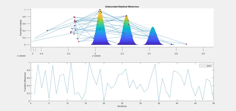
In the above grapth is can be seen that the inputs are boundless ga has mapped local maxima points outside our stalagmite function.The study time is very less as the ga is made only to run for the 50 iterations.
2.BOUNDED STATISTICAL BEHAVIOUR : (ITERATIONS = 100)
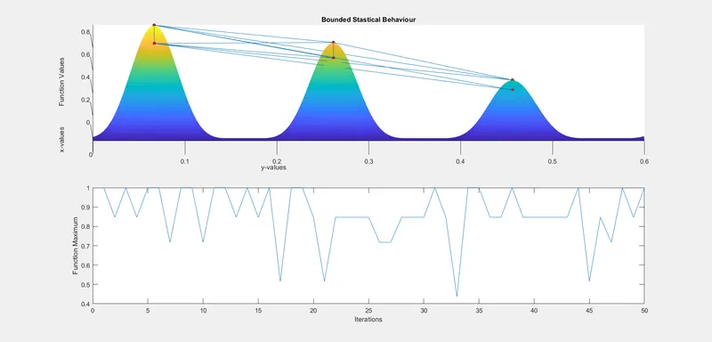
The above graph is clear and optimized compare to the first iterations since here the bounds were defined and we could get only the values within our range.
3.MODIFIED POPULATION SIZE PLOT: (ITERATIONS = 150)
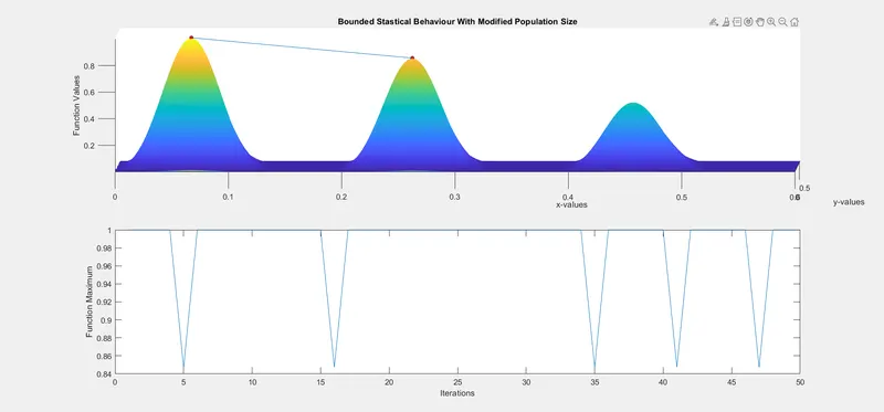
In this graph we ae geting the optimized value of global maxima with accurate range,since we increased the no.of iterations and population size. No of iterations and population size is increased the study time is so high compared to the previous two process.
It can be concluded that ga gives more accurate results in case of bounded inputs and by increasing the no.of iterations and population size.
OUTPUT PRINTED IN COMMAND WINDOW:
Study 1 : Unbounded Statistical Behaviour:
The time taken for the study 1 is : 3.242721
The coordinates of x & y for the global maximaof the function are : 0.2668469,0.259821
The global maxima of the function is : 0.512078
Study 2 : Bounded Statistical Behaviour:
The time taken for the study 2 is : 4.983019
The coordinates of x & y for the global maximaof the function are : 0.066833,0.261913
The global maxima of the function is : 0.984717
Study 3 : Bounded Statical Behaviour with Modified Populations:
The time taken for the study 3 is : 8.530761
The coordinates of x & y for the global maximaof the function are : 0.066833,0.066835
The global maxima of the function is : 0.998765
ERRORS DONE WHILE CODING:
1.
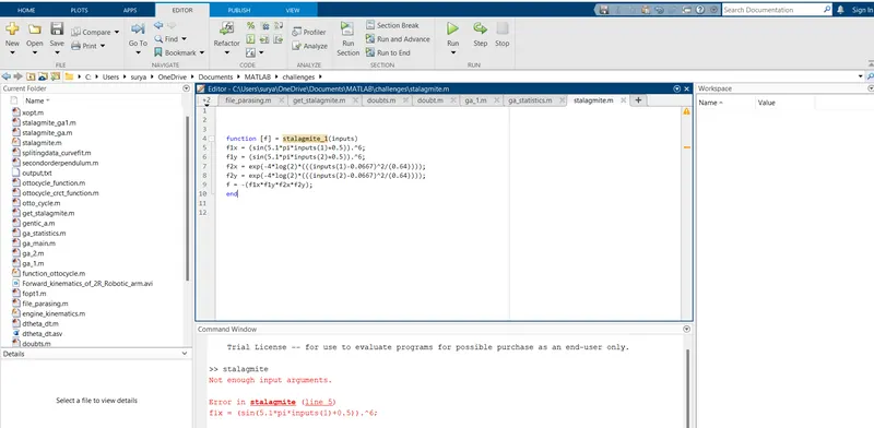
Made a mistake in function name. By seeing command window i rectified my errors.
2.

Assuming different variables in the main progra. By seeing the command window i rectifed my error.
3.
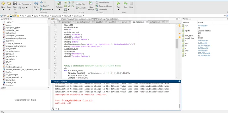
Typo errors are made while coding. All of them gets indicates in command window and by seeing that i rectife my errors.
OBSERVATION:
1.UNBOUNDED STATISTICAL BEHAVIOUR:
Time taken for the study_1 = 3.242721
The global maxima of the function is : 0.512078
2.BOUNDED STATISTICAL BEHAVIOUR:
The time taken for the study 2 is : 4.983019
The global maxima of the function is : 0.984717
3.BOUNDED STATISTICAL BEHAVIOUR WITH INCREASE POPULATION SIZE:
The time taken for the study 3 is : 8.530761
The global maxima of the function is : 0.998765
The total time taken to complete the total study = 16.956501
RESULTS:
Thus the Stalagmite function and to find Global Maxima of the function using Genitic Algorithm in MATLAB Programimng is performed.
REFERENCES: