To study the 'Genetic Algorithm' for optimising the stalagmite function.

Aim: To optimise the stalagmite function and find the global maxima of the function.

Objective: * To find global maxima.

* To explain the concept of genetic algorithm.

* plot graphs for all 3 studies and global maxima.

Theory:

STALAGMITE:

A stalagmite is an upward-growing mound of mineral deposits that have precipitated from water dripping onto the floor of a cave. Most stalagmites have rounded or flattened tips. There are many other types of mineral formations found in caves

GENETIC ALGORITHM:

A genetic algoritm are commonly used to generate high-quality solutions for optimization problems and search problems. In genetic algorithm it randomly analyzises the population determine its fitness of the population.If ga finds any missing data or any kind of error it will again select the population values and then it will crossover the value followed by mutation after all this if the value is good or fitness is good it will terminate the best result.

syntax for ga:

x = ga(fun,nvars)

x = ga(fun,nvars,A,b)

x = ga(fun,nvars,A,b,Aeq,beq)

x = ga(fun,nvars,A,b,Aeq,beq,lb,ub)

x = ga(fun,nvars,A,b,Aeq,beq,lb,ub,nonlcon)

x = ga(fun,nvars,A,b,Aeq,beq,lb,ub,nonlcon,options)

x = ga(fun,nvars,A,b,[],[],lb,ub,nonlcon,IntCon)

x = ga(fun,nvars,A,b,[],[],lb,ub,nonlcon,IntCon,options)

x= ga(problem)

[x,fval] = ga(___)

[x,fval,exitflag,output] = ga(___)

[x,fval,exitflag,output,population,scores] = ga(___)

Matlab coding for global maxima

% global maxima

clear all
close all
clc

x = linspace(0,0.8,150);
y = linspace(0,0.8,150);

%creating 3d mesh
[xx, yy] = meshgrid(x,y);

%evaluating stalagmite function

for i=1:length(xx)
    
    for j=1:length(yy)
        input_vector(1)=xx(i,j);
        input_vector(2)=yy(i,j);
        f(i,j)=stalagmite(input_vector);
        
    end
end

surfc(xx,yy,f)
xlabel('f maximum')
ylabel('interations')
shading interp
[inputs,fval] = ga(@stalagmite,2);

%global maxima

function [f] = stalagmite(input_vector)

x = input_vector(1);
y = input_vector(2);

f1 = (sin(5.1*pi*x+0.5))^6;
f2 = (sin(5.1*pi*y+0.5))^6;
f3 = exp(-4*log(2)*(x-0.0667)^2/0.64);
f4 = exp(-4*log(2)*(y-0.0667)^2/0.64);

f = (f1*f2*f3*f4);
end

Matlab coding for global minima:

%All 3 cases for global minima

clear all
close all
clc

x = linspace(0,0.8,150);
y = linspace(0,0.8,150);

%creating 3d mesh

num_cases = 50;
f=get_stalagmite(x,y);
tic
%study for case 1
for i=1:num_cases
    [inputs,fopt(i)]=ga(@stalagmite,2);
    xopt(i)=inputs(1);
    yopt(i)=inputs(2);   
end
start1_time=toc;
figure(1)
subplot(2,1,1)
surfc(x,y,f)
shading interp
hold on
plot3(xopt,yopt,fopt,'marker','o','markerfacecolor','r','markersize',5)
title('unbounded inputs')
subplot(2,1,2)
plot(fopt)
xlabel('iterations')
ylabel('f minimum')
tic
%study for case 2 with upper and lower bounds
for i=1:num_cases
    [inputs,fopt(i)]=ga(@stalagmite,2,[],[],[],[],[0;0],[1;1]);
    xopt(i)=inputs(1);
    yopt(i)=inputs(2);   
end
start2_time=toc;
figure(2)
subplot(2,1,1)
surfc(x,y,f)
shading interp
hold on
plot3(xopt,yopt,fopt,'marker','o','markerfacecolor','r','markersize',5)
title('unbounded inputs')
subplot(2,1,2)
plot(fopt)
xlabel('iterations')
ylabel('f minimum')

%study for case 2 increasing ga iterations
options = optimoptions('ga');
options = optimoptions(options,'PopulationSize',200);

tic
for i=1:num_cases
    [inputs,fopt(i)]=ga(@stalagmite,2,[],[],[],[],[0;0],[1;1],[],options);
    xopt(i)=inputs(1);
    yopt(i)=inputs(2);   
end
start3_time=toc;
figure(3)
subplot(2,1,1)
surfc(x,y,f)
shading interp
hold on
plot3(xopt,yopt,fopt,'marker','o','markerfacecolor','r','markersize',5)
title('unbounded inputs')
subplot(2,1,2)
plot(fopt)
xlabel('iterations')
ylabel('f minimum')

function [f] = get_stalagmite(x,y)

for i=1:length(x)
    for j=1:length(y)
        f1 = (sin(5.1*pi.*x(i)+0.5)).^6;
        f2 = (sin(5.1*pi.*y(j)+0.5)).^6;
        f3 = exp(-4*log(2).*(x(i)-0.0667).^2/0.64);
        f4 = exp(-4*log(2).*(y(j)-0.0667).^2/0.64);
         f(i,j) = -(f1.*f2.*f3.*f4);
    end
   
end

Explanation:

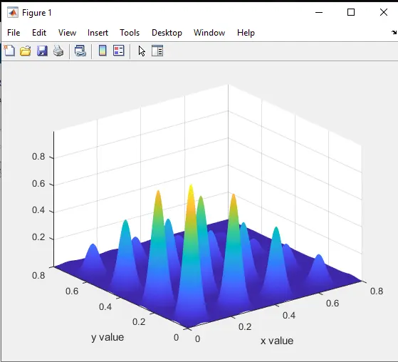
• First for global maxima we defined a search space be giving x and y values followed by we created 2d mesh of x and y.Then we used the forloop for evaluate the stalagmite function and wrote the function for x and y and put that values in given f1,f2,f3 and f4 equations.
• surfc syntax is used in this so that we can get 3d plot and shadin interp basically hides all the liines and give us the shaded part only and then we used ga syntax to call the stalagmite function.
• For 3 cases of global minima we gave first the numcases syntax to run ga syntax to defined number of times and then we called the get_stalagmite function which we wrote for solving minima functions.
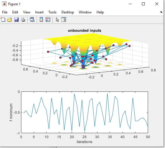
• For case 1 we called the ga function and ploted in figure 1 and by giving subplot syntax we got 1 row and 2 columns plot and followed by surfc syntax and we used plot3 syntax for getting 3 values to be plotted on the same graph and gave the title to the plot
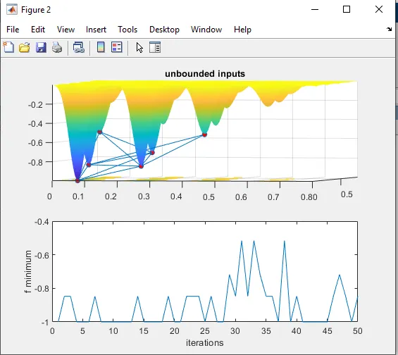
• For case 2 we gave the upper and lower bounds and in calling the function we gave simple blank square brackets non linearised values of a.b,aeq,beq and we got plot with some clearity but not much appropriate plot.
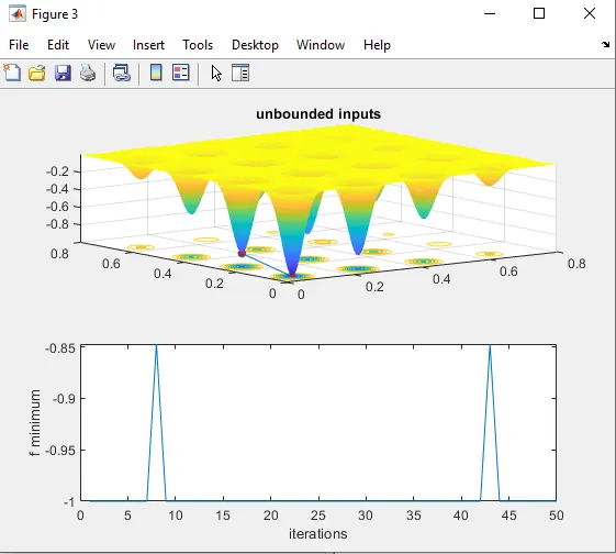
• For case 3 we gave the fixed population size by using optimoptions syntax and we got the clear plot of the minimas.

Output/Result:

Global maxima

All 3 cases for global minima: