Aim:- Write a code in MATLAB to optimise the stalagmite function and find the global maxima of the function.

Genetic Algorithm:- Genetic Algorithm (GA) is inspired by the process of Natural Selection.Genetic algorithms are commonly used to generate high-quality solutions to optimization and search problems by relying on biologically inspired operators such as mutation, crossover and selection.

Genetic Algorithms - Fundamentals

This section introduces the basic terminology required to understand GAs. Also, a generic structure of GAs is presented in both pseudo-code and graphical forms. The reader is advised to properly understand all the concepts introduced in this section and keep them in mind when reading other sections of this tutorial as well.

Basic Terminology

Before beginning a discussion on Genetic Algorithms, it is essential to be familiar with some basic terminology which will be used throughout this tutorial.

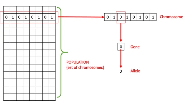
• Population − It is a subset of all the possible (encoded) solutions to the given problem. The population for a GA is analogous to the population for human beings except that instead of human beings, we have Candidate Solutions representing human beings.

• Chromosomes − A chromosome is one such solution to the given problem.

• Gene − A gene is one element position of a chromosome.

• Allele − It is the value a gene takes for a particular chromosome.

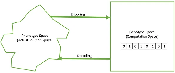
• Genotype − Genotype is the population in the computation space. In the computation space, the solutions are represented in a way which can be easily understood and manipulated using a computing system.

• Phenotype − Phenotype is the population in the actual real world solution space in which solutions are represented in a way they are represented in real world situations.

• Decoding and Encoding − For simple problems, the phenotype and genotype spaces are the same. However, in most of the cases, the phenotype and genotype spaces are different. Decoding is a process of transforming a solution from the genotype to the phenotype space, while encoding is a process of transforming from the phenotype to genotype space. Decoding should be fast as it is carried out repeatedly in a GA during the fitness value calculation.

  For example, consider the 0/1 Knapsack Problem. The Phenotype space consists of solutions which just contain the item numbers of the items to be picked.

  However, in the genotype space it can be represented as a binary string of length n (where n is the number of items). A 0 at position x represents that x^th item is picked while a 1 represents the reverse. This is a case where genotype and phenotype spaces are different.

• Fitness Function − A fitness function simply defined is a function which takes the solution as input and produces the suitability of the solution as the output. In some cases, the fitness function and the objective function may be the same, while in others it might be different based on the problem.

• Genetic Operators − These alter the genetic composition of the offspring. These include crossover, mutation, selection, etc.

The basic structure of a GA is as follows −

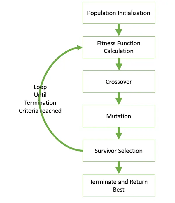
We start with an initial population (which may be generated at random or seeded by other heuristics), select parents from this population for mating. Apply crossover and mutation operators on the parents to generate new off-springs. And finally these off-springs replace the existing individuals in the population and the process repeats. In this way genetic algorithms actually try to mimic the human evolution to some extent.

Each of the following steps are covered as a separate chapter later in this tutorial.

Syntax for GA:-

stalagmite function:-Basically we created a code for stalagmite function using function

function A=stalagmite(input_vector)
x=input_vector(1);
y=input_vector(2);
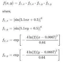
f1=(sin(5.1*pi*x+0.5)).^6;
f2=exp((-4*(log(2))*((x-0.0667).^2)/0.64));
f3=(sin(5.1*pi*y+0.5)).^6;
f4=exp((-4*(log(2))*((y-0.0667).^2)/0.64));
A=-(f1*f2*f3*f4);
end

Main function:-

clear all
close all
clc
x=linspace(0,0.6,150); -we created a 1-diamentional array of 150 values between 0 to 0.6 using linspace for x and y
y=linspace(0,0.6,150);
[xx,yy]=meshgrid(x,y); -we created a matrix of x&y ;we created a mesh
num_cases= 50; - GA will run 50 times
%Evaluating stalagmite function
for i=1:length(xx)
for j=1:length(yy)

input_vector(1)=xx(i,j);
input_vector(2)=yy(i,j);

input_vector=[input_vector(1),input_vector(2)]
GA(i,j)= stalagmite(input_vector); -calling the function created
end

end

Procedure:-

1)Start with usual commands clear all;close all;clc.Then we defined search space with two variables x&y.then we created one dimentional arrays for x & y using linspace command taking 150 values between 0 to 0.6.

2)Then we used for loop for we defined that we are creating two arrays input_vector1 & input_vector2 for each value of x & y and saved it in input_vector.

3) To calculate maxima we call stalagmite function.

4)This function is called in for loop & passing number of variables as input.for loop generates data for plot.

5)Doing 3 studies to get maximas

Study-1|Statistical behaviour|Unbounded condition

%%Study-1|Statistical behaviour|Unbounded condition
tic
for i=1:num_cases
          [input,GA_opt(i)]= ga(@stalagmite,2);
           xopt(i)=input(1);
           yopt(i)=input(2);
end
Study_1_time=toc
%Plotting the graph
figure(1)
subplot(2,1,1)
hold on
surfc(x,y,-GA)
%shading interp
plot3(input(1),input(2),-GA_opt,'marker','o','markersize',5,'MarkerFaceColor','r')
title('Unbounded inputs')
subplot(2,1,2)
plot(-GA_opt)
xlabel('Iteration')
ylabel('Function minimum')

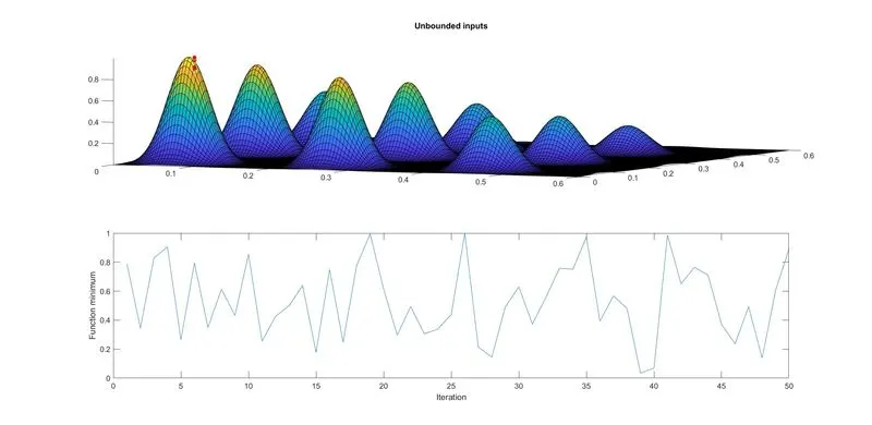
Explanation of study 1:-

After creating x,y variables input variables.

As the search space is not defined for GA. it does not know actual space & value of x&y will go above and below 0&0.6.

1) We run code for 50 times using for loop

Then we call ga and use the stalagmite function pass two variables as inputs and store its output in GA_opt.And store the values of x&y in xopt&yopt

2)To see the output , i use the surfc command we provide x ,y, function

then we create a 3D plot taking input(1) input(2) and -GA_opt and in sub plot we plot -GA_opt.

Study 2:-

%%Study-2|Bounded inputs
tic
for i=1:num_cases
          [input,GA_opt(i)]= ga(@stalagmite,2,[],[],[],[],[0;0],[2;2]);
           xopt(i)=input(1);
           yopt(i)=input(2);
end
Study_2_time=toc
%Plotting the graph
figure(2)
subplot(2,1,1)
hold on
surfc(x,y,-GA)
shading interp
plot3(input(1),input(2),-GA_opt,'marker','o','markersize',5,'MarkerFaceColor','r')
%plot3(xopt,yopt,-GA_opt,'marker','o','markersize',5,'MarkerFaceColor','r')
title('Bounded inputs')
subplot(2,1,2)
plot(-GA_opt)
xlabel('Iteration')
ylabel('Function minimum')

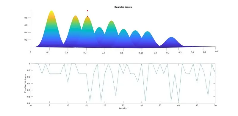
Explanation :- In study 2 we bounded the inputs.

Giveing x & y lower and upper limit a 0 and 2. Applying boundry conitions code will give us more perticular results.

Study 3:-

%%Study-3|Increasing GA Iterations|More no of population size
tic
options=optimoptions('ga','Populationsize',300)
for i=1:num_cases
[input,GA_opt(i)]= ga(@stalagmite,2,[],[],[],[],[0;0],[1;1],[],[],options);
xopt(i)=input(1);
yopt(i)=input(2);
end
Study_3_time=toc
%Plotting the graph
figure(3)
subplot(2,1,1)
hold on
surfc(x,y,-GA)
shading interp
plot3(xopt,yopt,-GA_opt,'marker','o','markersize',5,'MarkerFaceColor','r')
title('Study-3|Increasing GA Iterations|More no of population size')
subplot(2,1,2)
plot(-GA_opt)
xlabel('Iteration')
ylabel('Function minimum')

Explanation :-

In study 3 we increase the size of population. we increase the populaton size to 300 and we get the maxima in two peaks

and apply constrains in optimoptions and save its value in 'options' to allow GA to predict the optimum solution.

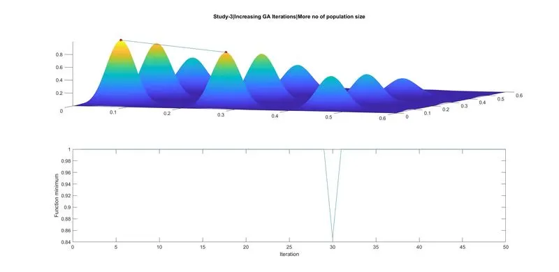
In the graph maxima lies around fist and second peak.It lies around 0.84.

increasing no. iteration and population size it takes more time than other studies.