Project 1 - Parsing NASA thermodynamic data

Aim:-

• Write a matlab program that take the "THERMO.dat" file as an input and generate Cp, H and S plots.
• Plot the Cp, Enthalpy and Entropy for the local temperature range (low temperature : high temperature) specific for each species.
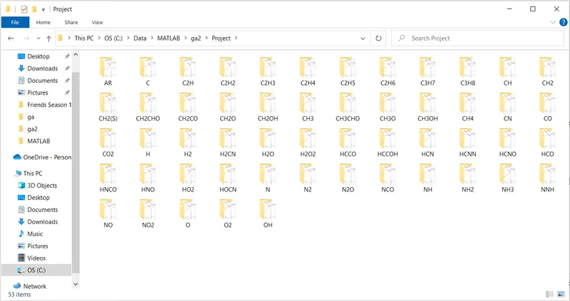
• Save the plots as images with appropriate names and dump them in separate folders for each species with suitable name. All these should be generated automatically.
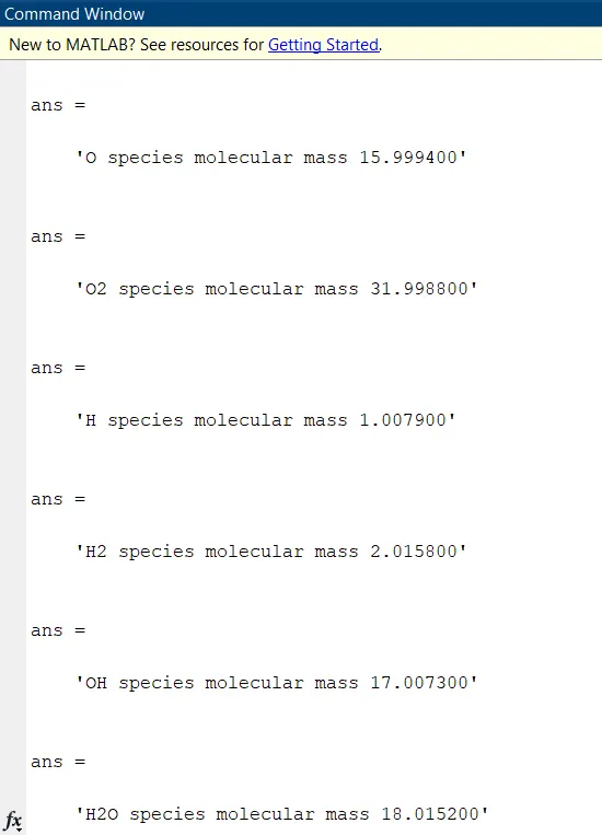
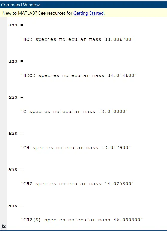
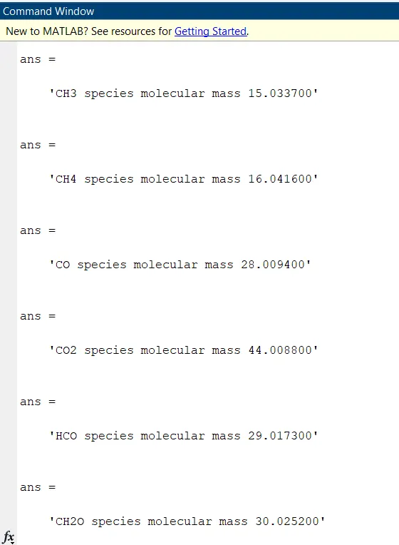
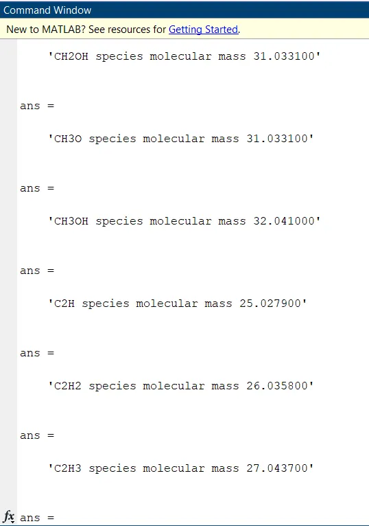
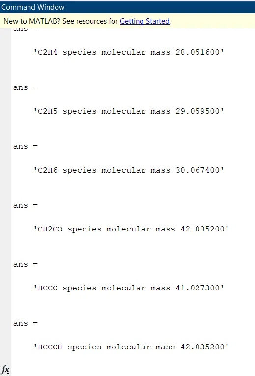
• Calculate the molecular weight of each species and display it in the command window.
• Write a detailed report to describe logic.

Main Program:-

clear all 
close all 
clc
f1= fopen('THERMO.dat','r');
gt=fgetl(f1);
%splitting the gt1 to convert it into number
gt1=fgetl(f1);
gt1=strsplit(gt1);
%coverting cell array into numbers
global_low_temp=str2num(gt1{2});
global_mid_temp=str2num(gt1{3});
global_high_temp=str2num(gt1{4});
%Reading comment line with for loop
for l=1:3;
    skip_line=fgetl(f1); %skipping comments
end
%%Readings main data
for j=1:53      %defining for loop for 53 species
    %extracting line with data
    line=fgetl(f1);
    %splitting
    line_split=strsplit(line,' ');
    % converting cell array in to numbers
    Local_low_temp=str2num(line_split{end-3});%reading local low temperature
    Local_high_temp=str2num(line_split{end-2});%reading local high temperature
    Local_mid_temp=str2num(line_split{end-1});%reading local mid temperature

    species_name=line_split{1}; % defining species name 

    Low_temp_range=linspace(Local_low_temp,Local_mid_temp,50);
    LT=Low_temp_range;
    High_temp_range=linspace(Local_mid_temp,Local_high_temp,50);
    HT=High_temp_range;

    %now we are getting cofficients from line 6 for calculate the
    %cofficients
    tline=fgetl(f1);
    %get location of E so we can find the cofficients
    a=findstr(tline,'E');
    %with the help of this we can find the cofficients
    %7 are high temperature cofficients
    a1=tline(1:a(1)+3);
    a1=str2double(a1);
    a2=tline(a(1)+4:a(2)+3);
    a2=str2double(a2);
    a3=tline(a(2)+4:a(3)+3);
    a3=str2double(a3);
    a4=tline(a(3)+4:a(4)+3);
    a4=str2double(a4);
    a5=tline(a(4)+4:a(5)+3);
    a5=str2double(a5);

% next a6 and a7 in next line
    tline_2=fgetl(f1);
    b=findstr(tline_2,'E');

    a6=tline_2(1:b(1)+3);
    a6=str2double(a6);
    a7=tline_2(b(1)+4:b(2)+3);
    a7=str2double(a7);
    %below 7 are low temperature cofficients
    a8=tline_2(b(2)+4:b(3)+3);
    a8=str2double(a8);
    a9=tline_2(b(3)+4:b(4)+3);
    a9=str2double(a9);
    a10=tline_2(b(4)+4:b(5)+3);
    a10=str2double(a10);
    % next a11 to  a14 in next line
    tline_3=fgetl(f1);
    c=findstr(tline_3,'E');
    a11=tline_3(1:c(1)+3);
    a11=str2double(a11);
    a12=tline_3(c(1)+4:c(2)+3);
    a12=str2double(a12);
    a13=tline_3(c(2)+4:c(3)+3);
    a13=str2double(a13);
    a14=tline_3(c(3)+4:c(4)+3);
    a14=str2double(a14);

    %Declaring universal gas constant
    R=8.314;
    %calculating cp,H,S.
    cp_high=(a1+a2.*HT+a3.*HT.^2+a4.*HT.^3+a5*HT.^4).*R;% specific heat for high temp
    cp_low=(a8+a9.*LT+a10.*LT.^2+a11.*LT.^3+a12*LT.^4).*R;% specific heat for low temp

    H_high=(a1+a2.*(HT./2)+a3.*(HT.^2./3)+a4.*(HT.^3./4)+a5*(HT.^4./5)+a6./HT).*R.*HT;% Enthalpy for high temp
    H_low=(a8+(a9.*LT)/2+(a10.*LT.^2)/3+(a11.*LT.^3)/4+(a12.*LT.^4)/5+a13./LT).*R.*LT;% Enthalpy for low temp

    S_high= (a1*log(HT)+a2.*HT+(a3.*HT.^2)/2+(a4.*HT.^3)/3+(a5*HT.^4)/4+a7);% Entropy for high temp
    S_low=(a8*log(LT)+a9.*LT+(a10.*LT.^2)/2+(a11.*LT.^3)/3+(a12.*LT.^4)/4+a14);%% Entropy for low temp
    
    %%Plotting the graphs
    % Specific Heat vs Temp
    figure(1);
    plot(LT,cp_low,'b','LineWidth',2)
    hold on
    plot(HT,cp_high,'r','LineWidth',2)
    title('Specific Heat vs Temp',species_name)
    xlabel('Temperature(K)')
    ylabel('Specific heat(J/K kg)')
    legend('low temperature','high temperature')
    grid on
    hold off
    %Enthalpy vs temp
    figure(2);
    plot(LT,H_low,'b','LineWidth',2)
    hold on
    plot(HT,H_high,'r','LineWidth',2)
    title('Enthalpy vs Temp',species_name)
    xlabel('Temperature(K)')
    ylabel('Enthalpy(J or KJ)')
    legend('low temperature','high temperature')
    grid on
    hold off
    %Entropy vs temp.
    figure(3);
    plot(LT,S_low,'b','LineWidth',2)
    hold on
    plot(HT,S_high,'r','LineWidth',2)
    title('Entropy vs Temp',species_name)
    xlabel('Temperature(K)')
    ylabel('Entropy(J/K)')
    legend('low temperature','high temperature')
    grid on
    hold off
% making folders  as per species name  
mkdir('C:Project',species_name);
%Assinging the path
path1=sprintf('C:/Data/MATLAB/ga2/Project/%s/temp_vs_cp.png',species_name);
path2=sprintf('C:/Data/MATLAB/ga2/Project/%s/temp_vs_enthalpy.png',species_name);
path3=sprintf('C:/Data/MATLAB/ga2/Project/%s/temp_vs_entropy.png',species_name);
%saving plot to apropriate paths with name n format
saveas(figure(1),path1);
saveas(figure(2),path2);
saveas(figure(3),path3);

%calling the molecular weight funtion n it will give us the molecular
%weight of every species in commannd window
Molecular_Wt=molecular_weight(species_name);

end
fclose(f1)

1. Use fopen command to read the file.
2. Skip 1st line using fgetl command as it is not required.
3. Next line contains global temperature ,using fgetl we store them in string.
4. All temp get stored in single string, we separate them using 'strsplit '.
5. And store them in global low temp,global low temp,global mid temp,global high temp.
6. Then we skip the comments using for loop.
7. From 6th line we have main data,sets of species with its temperature and 7 high and 7 low temperature coeffitients.
8. There are 53 of such sets of different species. So we run the for loop for 53 times.
9. Then we separate species name n local temperatures.
10. Next 3 lines in data file contain coeffitients which are required.For that read the respective line and use 'findstr' to locate E in each location( a=findstr(tline,'E');)
11. a1=tline(1:a(1)+3);will give us 1st coffitient,then store it in a1 [a1=str2double(a1);]
12. For coeffitient a2 we use a2=tline(a(1)+4:a(2)+3);it give second coffitient.
13. We use same logic for extracting all 14 coffitients.
14. After that we can do the calculations.
15. Define value of universal gas constant R.
16. Then give fomulas for separate low temp range and high temp range to calculate specific heat,enthalpy & entropy.
17. Then plot the results:in figure(1) plotted Specific Heat vs Temp; in figure(2) plotted Enthalpy vs Temp ; in figure(3) plotted Entropy vs Temp.
18. Then we created a directory using mkdir and giving it the path where we can create speparate folders and store plots of respective species.
19. using path we can name and give format to the plots.
20. Using saveas we save respective plots in folder with proper names.
21. After that call the molecular weight funtion n it will give us the molecular
    weight of every species in commannd window.

Molecular weight function:-

function Mol_Wt=molecular_weight(species_name)
%Mention all the species element in the 
element={'O','C','H','A','N','S'};
% atomic mass  of elements
Atomic_mass=[15.9994,12.01,1.0079,39.948,14.0067,32.065];
Mol_Wt=0;                                         % considering initial value of molecular weight as 0
for x=1:length(species_name)                      % Defining range of species lenghth in column
        for y=1:length(element)
            %strcmp compares s1 & s2 and return 1(true) if they are
            %idential else 0 (false)
            if strcmp(species_name(x),element(y)) %comparing two entities using if statement 
                Mol_Wt=Mol_Wt+Atomic_mass(y);     % add each molecular weight/atomic mass in every species 
                p=y;                              % it is stored in p
            end
        end
        q=str2num(species_name(x));               % convert all character array into atomic masses into number form
        if  q>1                                   %if atomic mass is more than 1  procide further
            Mol_Wt=Mol_Wt+Atomic_mass(p)*(q-1);   %molecular weight again calculated by species value (q-1)
    end
end

Outputs:-

1) folders of specific species:

2) molecular weight of species:-