Week 4.1 - Genetic Algorithm

Aim: To write a code in MATLAB to optimise the stalagmite function and find the global maxima of the function.

Stalagmite function:

A stalagmite is an upward-growing mound of mineral deposits that have precipitated from water dripping onto the floor of a cave. Stalagmite function generally refers to the function with which we are generating values over a stalagmite kind of surface for finding out the local and global maxima and minima of that particular given function.

Syntax for ga:

x = ga( fun , nvars , A , b , Aeq , beq , lb , ub )

here,

fun - Objective function

nvars - Number of variables

A,b - Linear inequality constraints

Aeq,beq - Linear equality constraints

lb - Lower bounds

ub - Upper bounds

Function:

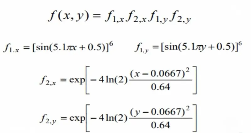
function f = stalagmite(input_vector)

x = input_vector(1);
y = input_vector(2);

f1x = (sin(5.1*pi*x + 0.5))^6;
f1y = (sin(5.1*pi*y + 0.5))^6;
f2x = exp(-4*log(2)*(x-0.0667)^2/0.64);
f2y = exp(-4*log(2)*(y-0.0667)^2/0.64);

f = -(f1x*f1y*f2x*f2y);
end

Program:

clear all
close all
clc

%Defining inputs to the solver
x = linspace(0,0.6,150);
y = linspace(0,0.6,150);
%let us run the Genetic Algorithm 50 times
num_cases = 50

[xx yy] = meshgrid(x,y);

%Evaluating the Stalagmite function
for i= 1:length(xx)
    for j = 1:length(yy)
        input_vector(1)=xx(i,j);
        input_vector(2)=yy(i,j);
        f(i,j) = stalagmite(input_vector);
    end
end

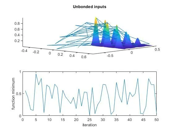
%Study 1 Statistical behaviour with unbonded behaviour
for i=1:num_cases
[results, min_val(i)] = ga(@stalagmite,2);
% ga is an in-built command
%'@stalamite' defines the function
% '2' denotes the number of variables in the function 
result_x (i)= results(1);
result_y(i) = results(2);
end

figure(1)
subplot(2,1,1)
hold on
surfc(xx,yy,-f)
shading interp
plot3(result_x,result_y,-min_val)
title('Unbonded inputs')
subplot(2,1,2)
plot(-min_val)
xlabel('iteration')
ylabel('function minimum')

 
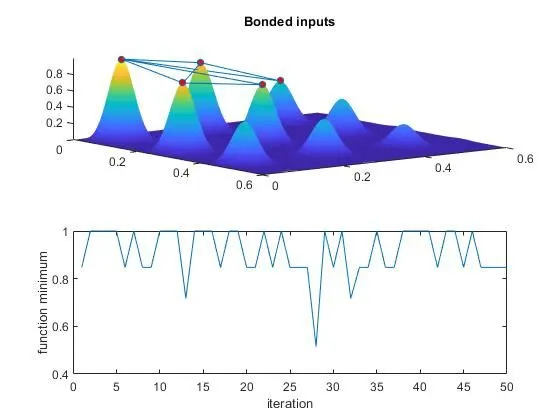
% Study 2 Statistical behaviour with bonded behaviour
tic
for i=1:num_cases
[results, min_val(i)] = ga(@stalagmite,2,[],[],[],[],[0;0],[1;1]);
result_x (i)= results(1);
result_y(i) = results(2);
end
time_2nd_iteration = toc


figure(2)
subplot(2,1,1)
hold on
surfc(xx,yy,-f)
shading interp
plot3(result_x,result_y,-min_val,'Marker','o','markersize',5,'markerfacecolor','r')
title('Bonded inputs')
subplot(2,1,2)
plot(-min_val)
xlabel('iteration')
ylabel('function minimum')


% Study 3 increasing GA interation

options = optimoptions('ga');
options = optimoptions(options,'PopulationSize',200);

% tic- toc command is used to measure the time taken to run the code within

tic
for i=1:num_cases
[results, min_val(i)] = ga(@stalagmite,2,[],[],[],[],[0;0],[0.1;0.1],[],[],options);
result_x (i)= results(1);
result_y(i) = results(2);
end
time_3rd_iteration = toc


figure(3)
%subplot command is used to divide the plot into desired parts
subplot(2,1,1)
hold on
surfc(xx,yy,-f)
shading interp
plot3(result_x,result_y,-min_val,'Marker','o','markersize',5,'markerfacecolor','r')
title('Bonded inputs with Modified population size')
subplot(2,1,2)
plot(-min_val)
xlabel('iteration')
ylabel('function minimum')

Explanation:

1. Defining the function.
2. And defining the inputs to the solver using linspace command.
3. Let us run the GA 50 times i.e. num_caes = 50.
4. Now evaluating the Salagmite function using for loop.
5. Study-1 is plotting the Statistical behaviour with unbounded behaviour.
6. Study-2 is plotting the Statistical behaviour bonded condition.
7. Study-3 is plotting the Statistical behaviour with certain population size and bounded condition.
8. Using 'surfc' command to plot 2D array and 'subplot' command to divide the plot into certain parts.
9. Using tic-toc command to capture the time between the codes.

Output:

Study 1:-

Study 2:-

Study 3:-

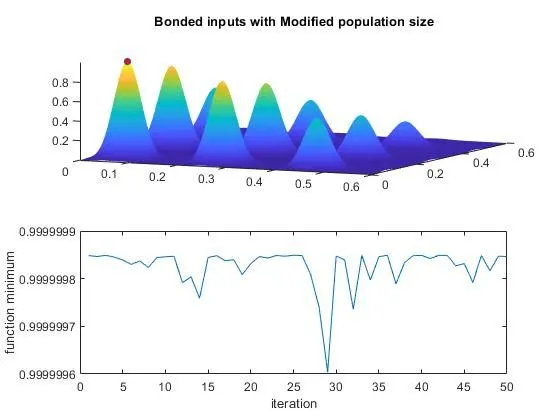
Conclusion: The red point in the study 3 is the global maxima of the function.