Week 3 - Solving second order ODEs

Simulation of Simple Harmonic Motion using Matlab

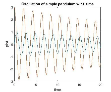
Aim: To plot the curve of the oscillation with respect to time of a simple pendulum and to obtain the motion in a 2D plain.

Breaking Down 2nd Order Differential equation:

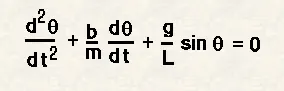
The way the pendulum moves depends on the Newtons second law. When this law is written down, we get a second order Ordinary Differential Equation that describes the position of the "ball" w.r.t time.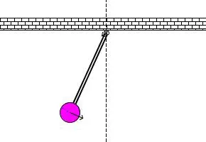

The command in the matlab which calculates the ODE is 'ode45'. This command can only calculate the first order differential equation.

In order to enter the equation into the program, first we need to break it down into two 1st order differential equations.

`if theta = theta_1`

`d theta/dt = d theta_1/dt = theta_2`

`d^2theta/dt^2=d^2theta_1/dt^2=d /dt(d theta/dt)= d theta_2/dt`

`d^2theta/dt^2+b/m d theta/dt+g/l sintheta = 0`

`d^2theta_1/dt^2+b/m d theta_1/dt+g/l sintheta_1 = 0`

`d theta_2/dt+b/m theta_2+g/l sintheta_1 = 0`

`d theta_1/dt = theta_2 and d theta_2/dt=-b/m theta_2-g/l sintheta_1`

`d/dt[theta_1 ;theta_2] = [theta_2;-b/m theta_2-g/l sintheta_1]`

Function program:

function [dtheta_dt] = ode_func(t,theta,b,g,l,m)
 

theta1 = theta(1)
theta2 = theta(2)
dtheta1_dt = theta2;
dtheta2_dt = -(b/m)*theta2 - (g/l)*sin(theta1);

dtheta_dt = [dtheta1_dt; dtheta2_dt];
 
end

Program to call Function:

clear all
close all
clc

%b=damping coefficient.
b = 0.05;
%g = gravity in m/s2,
g=9.81;
%L = length of the pendulum in m
l = 1;
%m = mass of the ball in kg
m = 1;

%angular displacement=0
%angular velocity=3 rad/sec
theta_0 = [0;3];

% the motion between 0-20 sec with 500 divisions
t_span = linspace(0,20,500);

[t, results] = ode45(@(t,theta) ode_func(t,theta,b,g,l,m),t_span,theta_0);

ct = 1;
for j = 1:length(results(:,1))
        
        x0 = 0;
        y0 = 1.1;
        
        y1 = -l*cos(results(j,1));
        x1 = l*sin(results(j,1));
          
       
        plot([x0 x1],[y0 y1],'linewidth',3)
        hold on
        plot(x1,y1,'o','MarkerFaceColor','red');
        hold off

        axis([-2 2 -2 2])
        title('Motion of a Simple Pendulum')
        xlabel('x-axis')
        ylabel('y-axis')
        grid on
        
        pause(0.09)
        M(ct) = getframe(gcf);
        ct=ct+1;


end

movie(M)

videofile = VideoWriter('ODE_2ND.avi','Uncompressed AVI')
open(videofile)
writeVideo(videofile,M)
close(videofile)


% for plotting the graph of the oscillation
plot(t,results(:,1))
hold on
plot(t,results(:,2))
title('Oscillation of simple pendulum w.r.t. time')
ylabel('plot')
xlabel('time')

Curve Obtained:

Pendulum Motion:

https://youtu.be/8PxA4mNvclU