Week 4.1 - Genetic Algorithm
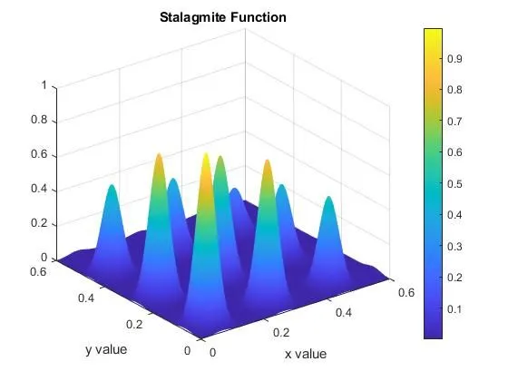
===> Stalagmite , this word indicates the formation of mountain surfaces naturally on earth, by this we will have maximum point and minimum point to describe and relate to some concepts to obtain the local maxima and global maxima values.
for finding an optimum solution by performing many iteration , we will be using Genetic Algorithm .
===> Genetic algorithm (GA) refers to method for solving both constarined and unconstrained optimization Problems based on a natural selection process. The algorithm repeatedly modifies a population of individual solutions at each step , the genetic algorithm randomly selects individual from current population and uses them a parents to produce the children for the next generation through successive generation, the population evolves towards an optimal solution.
Genetic algorithm uses the three main type of rules at each step to create the next generation from the current population. They are as follows.
1) Selection : this will select the individual called parents , that contribute to the population at the next generation , The selection function choose parents based on theie scaled values from the fitness scaling function. The scaled fitness values are called as exception values. An individual can be selected more than one time as a parent , in which it contributes its genes for more than one child.
2)Crossover : This will combine two parents to form childre for the next generation. The algorithm creates crossover child by combining pairs of Parents in the current population.
3)Mutation : This will apply random changes to the individual parents to form Children. The algorithm Creates Mutation children by randomly changing the genes of individual Parents.
'ga' is built in function in MATLAB which finds minimum of function using Genetic algorithm.
1) x=ga(fun,nvars): This finds a local unconstrained minimum, x ,x to the objective function, fun.nvars is the dimension( number of design variables) of fun.
2) x=ga(fun,nvars,A,b):Finds a local minimum x to fun , subject to the linearinequalities A*x<=b. 'ga' evaluates the matrix product A*x as if x is transposed (A*x').
3) x=ga(fun,nvars, A,b, Aeq,beq): Finds a local minimum x to fun , subject to the linear equalities Aeq*x=beq and A*x<=b. (Set A=[] and b=[] if no li9near inequalities exist.) ga evaluates the matrix product Aeq*x as if x is tranposed (Aq*x').
) )4) x=ga(fun,nvars,Aeq,beq,lb,ub):Defines a set of lower and upper bounds on the design variables , x so that a solution is found in the range lb<=x<=ub. ( Set Aeq=[] and beq=[] if no linear equalities exist.)
5) x=ga(fun,nvars,A,b,Aeq,beq,lb,ub,nonlcon): Subjects the minimization to the constraints defines in nonlcon. The function nonlcon accepts x and returns Vectors C and Ceq , representing the nonlineaer inequalities and equalities respectively. ga minimizes the fun such that C(x)<=0 and Ceq(x)=0. (Set lb=[] and ub=[] if no bounds exist.)
6) x=ga(fun,nvars,A,b,Aeq,beq,lb,ub,nonlcon,options) : Minimizes with the default optimization parameters replaced by values in options. (Set nonlcon=[] if no nonlinear constraints exist.) Create options using optimoptions.
7)x=ga(fun,nvars,A,b,[],[],lb,ub,nonlcon,intCon) or x=ga(fun,nvars,A,b,[],[],lb,ub,nonlcon,IntCon, options): Requirs that the varible listed in IntCon take integer values.
8) x=ga(problem): Finds the minimum for problem, where problem is a structure.
9)[x,favl] = ga(___): For any previous input arguments , also returns fval, the value of the fitness at x.
10) [x,fval,exitflag,output]=ga(___): Alsoreturns exitflag, an integer identifying the reason the algorithm terminated , and output , a structure that contains output from each generation and other information about the performance of the algorithm.
11) [x,fval,exitflag,output,population,scores]=ga(___): Also returns a matrix population , whose rows are the final population, and a vector scores, the scores of the final population.
PROGRAM for stalagmite function is as follows :
function[f] = stalagmite_function(input_vector)

x = input_vector(1);
y = input_vector(2);

term1 = (sin((5.1*pi*x)+0.5))^6;

term2 = (sin((5.1*pi*y)+0.5))^6;

term3 = exp(-4*log(2)*((x-0.0667)^2)/0.64);

term4 = exp(-4*log(2)*((y-0.0667)^2)/0.64);

f = -(term1*term2*term3*term4);

end
Here for calculating calculating maximum value we are multiplying with (-).
The below program is to optimize the stalagmite function by using Genetic Algorithm.
clear all
close all
clc

%Defining our search space
x=linspace(0,0.6,150);
y=linspace(0,0.6,150);
n=50;

%Creating 2D mesh
[xx yy] = meshgrid(x,y);

%Evaluating stalagmite function

for i=1:length(xx)
    for j=1:length(yy)
        input_vector(1)=xx(i,j);
        input_vector(2)=yy(i,j);
        f(i,j)= stalagmite_function(input_vector);
    end
end
%   Plotting the stalagmite function
figure(1)
surf(xx,yy,-f)
shading interp
xlabel('x value')
ylabel('y value')
title('Stalagmite Function')
colorbar

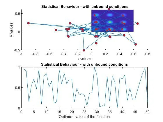
%case1 - Statistical Behaviour (with unbound conditions)
tic    %stating the time count

for k=1:n
    [inputs1 ,fopt1(k)] = ga(@stalagmite_function, 2);

    %Using "ga" to optimize the function for maximum value
    %fopt1 contains value of the function at the particular inputs1 which
    %has x and y co-ordinates for current iteration

    xopt1(k) = inputs1(1);
    yopt1(k) = inputs1(2);
end

time1 = toc  %Stopping time count and storing the time required for all the iteration in time1
%Plotting
figure(2)
subplot(2,1,1)
hold on
surf(xx,yy,-f) %creating a 3D plot of the Stalagmite function
shading interp  % Turning off the grid

%Plotting the optimum ponts produced by genetic algorithm performed on
%stalagmite function

plot3(xopt1 , yopt1 , -fopt1 , 'marker','o','markerfacecolor','r')
xlabel('x values')
ylabel('y values')
title(' Statistical Behaviour - with unbound conditions')

%Plotting the optimim value produced with each iteration
subplot(2,1,2)
plot(-fopt1)
xlabel('Optimum value of the function')
title('Statistical Behaviour - with unbound conditions')

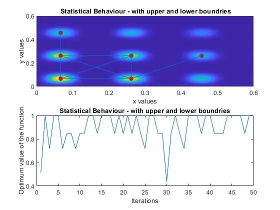
%case2- Statistical Behaviour - with upper and lower bound
tic   %Starting the time count
for k = 1:n
    [inputs2 , fopt2(k)]= ga(@stalagmite_function, 2 ,[],[],[],[],[0;0],[1;1]);


    %Using "ga" to optimize the function for maximum value
    %fopt2 contains value of the function at the particular inputs1 which
    %has x and y co-ordinates for current iteration
    xopt2(k) = inputs2(1);
    yopt2(k)= inputs2(2);
end
time2= toc  %Stopping time count and storing the time required for all the iteration in time1
%Plotting
figure(3)
subplot(2,1,1)
hold on
surf(xx,yy,-f) %creating a 3D plot of the Stalagmite function
shading interp  % Turning off the grid

%Plotting the optimum ponts produced by genetic algorithm performed on
%stalagmite function

plot3(xopt2 , yopt2 , -fopt2 , 'marker','o','markerfacecolor','r')
xlabel('x values')
ylabel('y values')
title(' Statistical Behaviour - with upper and lower boundries')

%Plotting the optimim value produced with each iteration
subplot(2,1,2)
plot(-fopt2)
xlabel('Iterations')
ylabel('Optimum value of the function')
title('Statistical Behaviour - with upper and lower boundries')

%%Case 3 - Statistical Behaviour - with inceasing GA iterations

options = optimoptions('ga'); %This line specifies that th options is to be given to ga function.
options = optimoptions(options,'populationsize',300); %This line specifies that the population size will be 300.

tic %starting the time count

for k =1:n
    [inputs3 , fopt3(k)]= ga(@stalagmite_function, 2 ,[],[],[],[],[0;0],[1;1],[],[],options);
    %Using "ga" to optimize the function for maximum value
    %fopt2 contains value of the function at the particular inputs1 which
    %has x and y co-ordinates for current iteration
    xopt3(k)=inputs3(1);
    yopt3(k)=inputs3(2);

end
time3= toc  %Stopping time count and storing the time required for all the iteration in time1
%Plotting
figure(4)
subplot(2,1,1)
hold on
surf(xx,yy,-f) %creating a 3D plot of the Stalagmite function
shading interp  % Turning off the grid

%Plotting the optimum ponts produced by genetic algorithm performed on
%stalagmite function

plot3(xopt3 , yopt3 , -fopt3 , 'marker','o','markerfacecolor','r')
xlabel('x values')
ylabel('y values')
title(' Statistical Behaviour - with increased Ga iterations')

%Plotting the optimim value produced with each iteration
subplot(2,1,2)
plot(-fopt3)
xlabel('Iterations')
ylabel('Optimum value of the function')
title(' Statistical Behaviour - with increased Ga iterations')

x_point = [xopt1(50);xopt2(50);xopt3(50)];
y_point = [yopt1(50);yopt2(50);yopt3(50)];
optimum_value = [-fopt1(50);-fopt2(50);-fopt3(50)];
time_taken = [time1;time2;time3];

names = {'Statistical Behaviour - with unbound conditions' ; 'Statistical Behaviour - with upper and lower boundaries'; ' Statistical Behaviour - with increased GA iterations'};

tab = table(x_point, y_point,optimum_value,time_taken,'RowNames',names)
Explanation :
1) In the first steps we are defining the stalagmite function based on its nature. Then for grtting optimized value for the function , we are using genetic algorith with different syntax of inputs for better optimization results.
2) we are going to perform the genetic algorithm in the name of three cases , where we will be using more optimized syntax for the appropriate results.
3) in case 1 we are not specifyning any boundaries and the optimesed input values from the iteration and also function value can be calculated in certain time period.
4) in case 2 , we are giving certain boundaries ( upper and lower boundaries to facilitate the algorithm to give the output with more optimezed values than the case1.
5) in case 3 we are adding more changes to the syntx , where the algorithm finds the Population of size beyond the specified iterations with which no of iteration can be increased for better results in findng the optimim values i.e global maxima of the function at the respective co-ordinate points.
6) in each case we are making the subplt options to show the combined results for optimum values for co-ordnates and also the optimum value results against the respective iterations.
The plotting results are as follows.
Stalagmite plot :
case1 results ( without the specified boundaries):
case2 results : with upper and lower Boundaries :
case3 : with more iteration where the Genetic algorithm uses more and more crossover or mutations rules with lage space of population.:
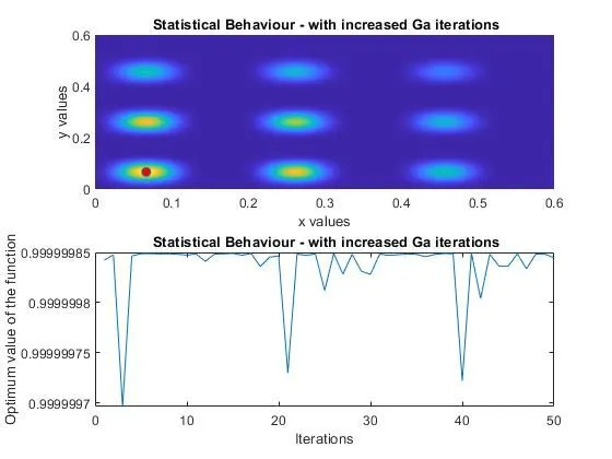
As we can see that there is a minor deviation in the obtained results for the stalagmite function in case 3.
variable outputs :
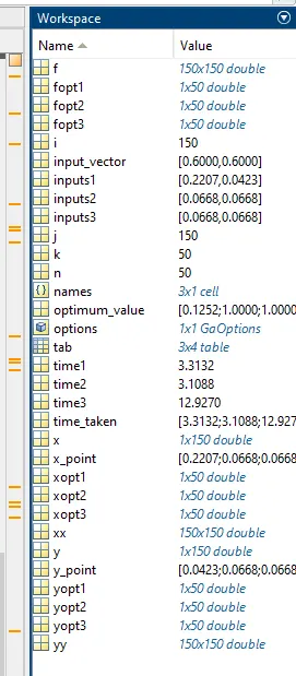
The main results we can see here is , at each case the genetic algorithm gives values for inputs and fopt values from its operations. these are the major and needed outputs for the stalagmite function.
Summarised Output:
                                                         x_point     y_point     optimum_value    time_taken
                                                               ________    ________    _____________    __________

    Statistical Behaviour - with unbound conditions             0.22066    0.042258       0.12519         3.3132
    Statistical Behaviour - with upper and lower boundaries    0.066844    0.066829             1         3.1088
    Statistical Behaviour - with increased GA iterations       0.066831    0.066834             1         12.927
ERRORS ENCOUNTER :
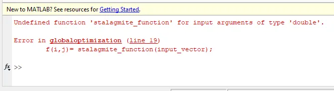
ERROR1: When you define the function , and you are running actual progam . in mean while if you run some other query program, then the defined function will not be shown as defined i believe. So just save your actual code and re-open the matlab , later run the program.
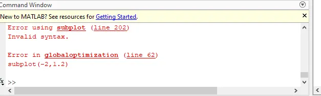
ERROR 2 : This is like a typo error when i am writing the subplot syntax without knowing the actual meaning of it.
so detailed study is required before using any type of syntax what they actually mean and what they neded for the expected output.
THANK YOU.