Project 2 - Rankine cycle Simulator
RANKINE CYCLE : This cycle involves coverting thermal energy into Mechanical Energy which will be used to generate Electrical energy ( Mainly in Thermal Power plants ) . Rankine cycle is named after him. In this cycle the fluid used is mainly water . The water is given a constant pressure heat addition in the boiler and is coverted to steam which passes over the turbines with expanding nature and turning the turbine blades ( mechanical work) and then generating Electrical energy.
There are many properties of water that makes this cycle to select it as a fluid for the system. As it undergoes phase changes ( liquid <--->Vapour) with minor losses and giving a good value of efficiency .
Rankine cycle consists of mainly four processes ( Two isentropic and two isobaric ), They ae as follows
Process 1 - 2 : Isentropic Expansion in a turbine
Process 2 - 3 : constant pressure heat rejection in condenser
Process 3 - 4 : Isentropic compression in the pump
Process 4 - 1 : Constant Pressure heat addition in the boiler.
MATLAB Code for RANKINE CYCLE
clear all
close all
clc

disp('RANKINE CYCLE')

disp('1-2 is isentropic expansion in the Turbine');
disp('2-3 is Constant pressure heat removal in the Condenser');
disp('3-4 is isentropic compression in the pump');
disp('4-1 is constant pressure heat addition in the boiler');


p1 = input('nValue of pressure at turbine inlet , p1(in bar) = ');
T1 = input('nValue of temperature at turbine inlet, T1(in degree.C)= ');
p2 = input('nValue of pressure at condensor inlet, p2(in bar) = ');

%At state 1
h1 = XSteam('h_pT',p1,T1);   %Extracting Enthalpy at state pt 1
s1 = XSteam('s_pT',p1,T1);   %Extracting Entropy at state pt 1

%At state 2                   %Isentropic expansion
s2 = s1;
sf2 = XSteam('sL_p',p2);      %Saturated Liquid Entropy
sg2 = XSteam('sV_p',p2);      %Saturated Vapour Entropy
x2 = (s2-sf2)/(sg2-sf2);
hf2 = XSteam('hL_p',p2);
hg2 = XSteam('hV_p',p2);
h2 = hf2+(x2*(hg2-hf2));

%At state 3                  %Constant pressure heat Rejection
p3 = p2;
s3 = XSteam('sL_p',p3);
h3 = XSteam('hL_p',p3);

%At state 4
s4 = s3;
p4  = p1;

%Work done by Turbine
Wt = h1-h2;

%Work done to run Pump
v3 = XSteam('vL_p',p3);  %Saturated Liquid Volume ( Specific volume)
Wp = v3*(p4-p3)*100;
h4 = h3+ Wp;

%Net Work
Wnet = Wt-Wp;

%Heat into the system
Qin = h1-h4;

%Heat out of thr system
Qout = h2-h3;

%Thermal Efficiency
thermal_eff = (Wnet/Qin)*100;

%Spcific Steam Consumption
%SSC = mass flow rate/power
SSC = (3600/Wnet);

%Back Work Ratio
BW = (Wp/Wt);

%Calculation of Temperatures at the state points
T3 = XSteam('Tsat_p',p3);
T2 = T3;
Cp4 = XSteam('Cp_ps',p4,s4);
Cv4 = XSteam('Cv_ps',p4,s4);
k = Cp4/Cv4 ;
T4 = T3/((p3/p4)^((k-1)/k));

%Calculating Temperature , Entropy and Enthalpy at the vapour and liquid
%line for plotting

T6 = XSteam('Tsat_p',p1);
s5 = XSteam('sL_p',p1);
s6 = XSteam('sV_p',p1);
h5 = XSteam('hL_p',p1);
h6 = XSteam('hV_p',p1);
T5 = T6;

%Plotting the saturation Curve

T = linspace(1,375,1000);
for i = 1:length(T)

    sf(i) = XSteam('sL_T',T(i));
    sg(i) = XSteam('sV_T',T(i));
    hf(i) = XSteam('hL_T',T(i));
    hg(i) = XSteam('hV_T',T(i));
end

%Plotting T-S Diagram
figure(1)
hold on
plot(sf,T,'r','linewidth',1)
plot(sg,T,'r','linewidth',1)
plot([s1 s2],[T1 T2], 'b','linewidth',2)
plot([s2 s3],[T2 T3], 'b','linewidth',2)
plot([s3 s4],[T3 T4], 'b','linewidth',2)
plot([s4 s5],[T4 T5], 'b','linewidth',2)
plot([s5 s6],[T5 T6], 'b','linewidth',2)
sc1 = linspace(s6,s1,1000);
for l = 1:length(sc1)
    Tc1(l) = XSteam('T_ps' ,p1 ,sc1(l));
end
plot(sc1, Tc1 , 'b','linewidth',2)
text(s1+0.1 , T1,'1')
text(s2+0.1 , T2,'2')
text(s3 , T3-20,'3')
text(s4 , T4+20,'4')

title('Temp vs Entropy plot')
xlabel('Entropy, S (Kj/kgk')
ylabel('Temperature (degree C)')
legend('Saturation curve')

%Plotting h-s diagram
figure(2)
hold on
plot(sf,hf, 'k','linewidth',1)
plot(sg,hg, 'k' ,'linewidth',1)
plot([s1 s2],[h1 h2],'r','linewidth',2)
plot([s2 s3],[h2 h3],'r','linewidth',2)
plot([s3 s4],[h3 h4],'r','linewidth',2)
hc = linspace(h4,h5,100);
for r=1:length(hc)
    sch(r) = XSteam('s_ph',p1,hc(r));
end
plot(sch,hc, 'r','linewidth',2)
plot([s5 s6],[h5 h6], 'r','linewidth',2)
for m = 1:length(sc1)
    hc1(m) = XSteam('h_ps',p1,sc1(m));
end
plot(sc1,hc1,'r','linewidth',2)
text(s1+0.1,h1,'1')
text(s2+0.1,h2,'2')
text(s3,h3-100,'3')
text(s4,h4+200,'4')
title('Enthalpy vs Entropy plot')
xlabel('Entropy , S(KJ/kgk)')
ylabel('Enthalpy , H (KJ/kg)')
legend('Saturation curve','location','northwest')


%Displaying the results in the Command Window:
disp('Results');
p1 = p1;
T1 = T1;
p2 = p2;

disp('At stage point 1');
n1 = sprintf('P1 is %.3f bar',p1);
disp(n1);
n2 = sprintf('T1 is %.3f C',T1);
disp(n2);
n3 = sprintf('h1 is %.3f KJ/kg',h1);
disp(n3);
n4 = sprintf('s1 is %.3f kJ/KgK',s1);
disp(n4);

disp('At stage point 2');
n11 = sprintf('P2 is %.3f bar',p2);
disp(n11);
n21 = sprintf('T2 is %.3f C',T2);
disp(n21);
n31 = sprintf('h2 is %.3f KJ/kg',h2);
disp(n31);
n41 = sprintf('s2 is %.3f kJ/KgK',s2);
disp(n41);

disp('At stage point 3');
n12 = sprintf('P3 is %.3f bar',p3);
disp(n12);
n22 = sprintf('T3 is %.3f C',T3);
disp(n21);
n32 = sprintf('h3 is %.3f KJ/kg',h3);
disp(n32);
n42 = sprintf('s3 is %.3f kJ/KgK',s3);
disp(n42);

disp('At stage point 4');
n13 = sprintf('P4 is %.3f bar',p4);
disp(n13);
n23 = sprintf('T4 is %.3f C',T4);
disp(n23);
n33 = sprintf('h4 is %.3f KJ/kg',h4);
disp(n33);
n43 = sprintf('s4 is %.3f kJ/KgK',s4);
disp(n43);


n14 = sprintf('Wt is %.3f kJ/Kg',Wt);
disp(n14);

n15 = sprintf('Wp is %.3f kJ/Kg',Wp);
disp(n15);


n16 = sprintf('Wnet is %.3f kJ/Kg',Wnet);
disp(n16);

n17 = sprintf('Thermal_efficiency is %.2f Percent',thermal_eff);
disp(n17);
n18 = sprintf('SSC is %.2f kg/KWh',SSC);
disp(n18);
n19 = sprintf('Back work ratio is %.3f',BW);
disp(n19);
Explanation :
1. Firstly for loading the values of Enthalpy , Entropy , specific volume , and some other thermal properties from XSteam data file for the water at saturated liquid and vapour conditions.
2. At each state points , we need to find the values of temperature , enthalpy and entropy by appling appropriate Thermal conditions , and also the available data from XSteam data file.
3. Extracting data for Temperature , enthalpy and entropy from Xsteam data file at liquid and vapour states.
4. Now calaculating sf,sg,hf,hg ( from Xsteam) , where f and g indicates saturated liquid and saturated vapour states, Finding the positions from rankine cycle and extracting the same from Xsteam.
5.Net work done , work done by turbine , work done for Pumping the fluid , Heat in and Heat out are calculated by using appropriate thermal conditions.
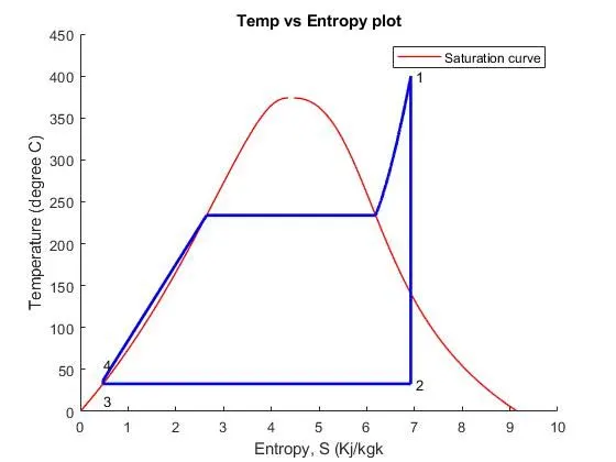
6. Now plotting between Tempearature and Entropy along with the Saturation line plot for the complete cycle with respect to temperature.
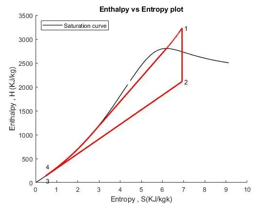
7. Now plotting between Entropy and Enthalpy along with the Saturation line plot for the complete cycle with respect to Enthalpy.
8. Results are dispalyed by using sprintf command.
Results :
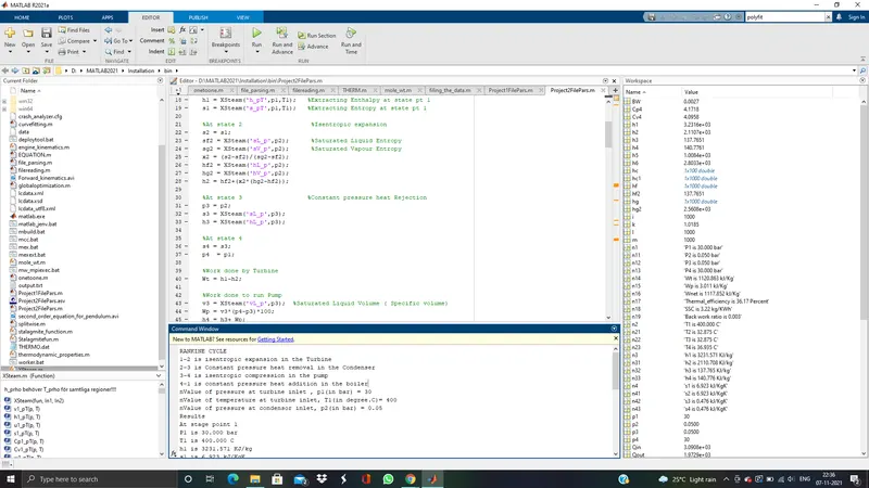
1)
2)
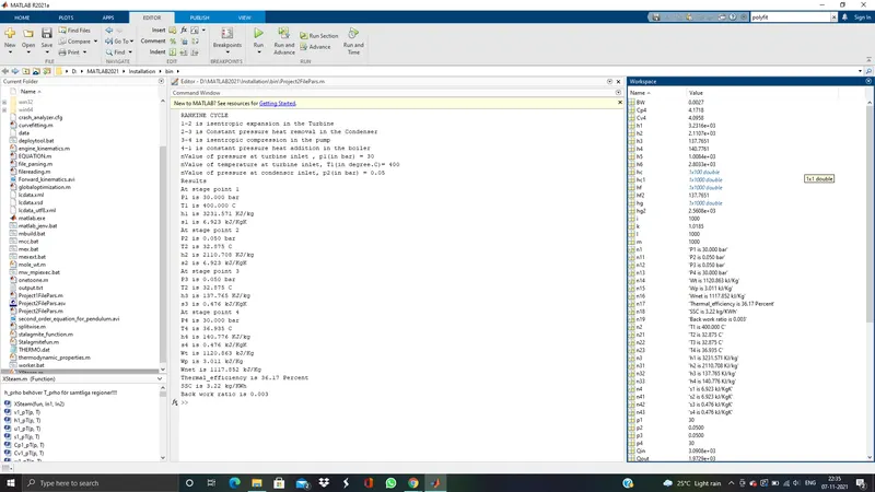
3) T-S plot
4) H -S Plot
Variable results ;
Wnet is 1117.852 kJ/Kg
Thermal_efficiency is 36.17 Percent
SSC is 3.22 kg/KWh
Back work ratio is 0.003
References :
1) https://medium.com/@ashwinpalo/how-to-calculate-thermal-efficiency-of-rankine-cycle-37a7dbcadc12
2) https://www.sciencedirect.com/topics/earth-and-planetary-sciences/rankine-cycle