Week 4.1 - Genetic Algorithm
Objective
- Write a code in MATLAB to optimise the stalagmite function and find the global maxima of the function.
- Clearly expalin the concept of genetic algorithm in your own words and also explain the syntax for ga in MATLAB.
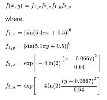
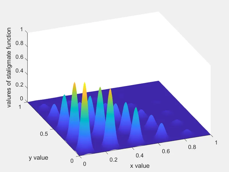
Stalagmite function:
Genatic Algorithom:
The Genatic algorithm was created based on the concept of natural selection theory. Natural selection is a biological theory was first proposed by Charles Darwin. In natural selection theory the organisms with high ability is qualified to survive in the current environment and generates new organisms into the new generation.
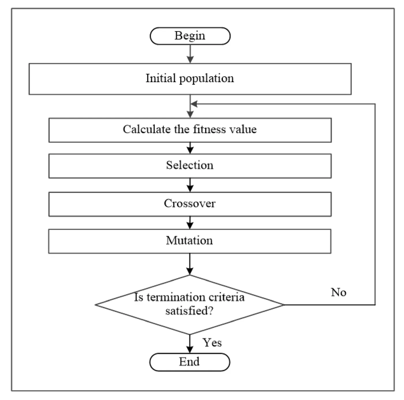
- First of all create an inetial population
- Then scores each member of the current population by computing its fitness value. These values are called the raw fitness scores.
- Scales the raw fitness scores to convert them into a more usable range of values. These scaled values are called expectation values.
- Selects members, called parents, based on their expectation.
- Some of the individuals in the current population that have lower fitness are chosen as elite. These elite individuals are passed to the next population.
- Produces children from the parents. Children are produced either by making random changes to a single parent mutation or by combining the vector entries of a pair of parents crossover.
- Replaces the current population with the children to form the next generation.
- The algorithm stops when one of the stopping criteria is met.
GA Syntax:
set 1
x = ga(fun,nvars)
x = ga(fun,nvars,A,b)
x = ga(fun,nvars,A,b,Aeq,beq)
x = ga(fun,nvars,A,b,Aeq,beq,lb,ub)
x = ga(fun,nvars,A,b,Aeq,beq,lb,ub,nonlcon)
x = ga(fun,nvars,A,b,Aeq,beq,lb,ub,nonlcon,options)
x = ga(fun,nvars,A,b,Aeq,beq,lb,ub,nonlcon,intcon)
x = ga(fun,nvars,A,b,Aeq,beq,lb,ub,nonlcon,intcon,options)
set 2
[x, fval] = ga(any one of the set 1)
[x, fval,exitflag,output] = ga(any one of the set 1)
[x, fval,exitflag,output,population,score] = ga(any one of the set 1)
x - local minimum
fun - given function
nvars - number of variables
A,b,Aeq,beq - linear equalities and inequalities
lb,ub - lower bounds and upper bounds
nonlcon,intcon - nonlinear equalities and inequalities
options - it used to change the fixed function tolerance
fval, the value of the fitness function at x
Code
close
clear
clc


% All inputs

x = linspace(0,1,150);
y = linspace(0,1,150);
[xx, yy] = meshgrid(x, y);
number_of_cases = 150;

% function inetializing

f=ones(length(x), length(y));
fopt = ones(number_of_cases,number_of_cases);
xopt = ones(number_of_cases,number_of_cases);
yopt = ones(number_of_cases,number_of_cases);
xoptim = ones(number_of_cases,number_of_cases);
yoptim = ones(number_of_cases,number_of_cases);
foptim = ones(number_of_cases,number_of_cases);
fop = ones(number_of_cases,number_of_cases);
xop = ones(number_of_cases,number_of_cases);
yop = ones(number_of_cases,number_of_cases);


for i = 1 : length(xx)
    for j = 1 : length(yy)
        input(1) = xx(i,j);
        input(2) = yy(i,j);
        f(i, j) = fun(input);
    end
end

figure(1)
surface(xx, yy, -f)
shading interp
xlabel('x value')
ylabel('y value')
zlabel('valures of staligmate function')
[output, fval] = ga(@fun, 2);


% case 1


for i = 1 : number_of_cases
     [inputs , fopt(i)] = ga(@fun, 2);
     xopt(i) = inputs(1);
     yopt(i) = inputs(2);
end


% plotting

figure(2)
subplot(2,1,1)
hold on
surfc(x,y,-f)
shading interp
plot3(xopt,yopt,-fopt,'marker','*')
xlabel('x value')
ylabel('y value')
zlabel('valures of staligmate function')
title('Case 1')
subplot(2,1,2)
plot(-fopt)
xlabel('cases(iterations)')
ylabel('Maximum values')


% case 2

for i = 1 : number_of_cases
    [in, foptim(i)] = ga(@fun,2,[],[],[],[],[0;0],[1;1]);
    xoptim(i) = in(1);
    yoptim(i) = in(2);
end

% plotting

figure(3)
subplot(2,1,1)
hold on
surfc(x,y,-f)
shading interp
xlabel('x value')
ylabel('y value')
zlabel('valures of staligmate function')
plot3(xoptim,yoptim,-foptim,'marker','*')
title('Case 2')
subplot(2,1,2)
plot(-foptim)
xlabel('cases(iterations)')
ylabel('Maximum values')


% case 3

options = optimoptions('ga');
options = optimoptions(options,'populationsize',300);

for i = 1 : number_of_cases
    [inp, fop(i)] = ga(@fun,2,[],[],[],[],[0;0],[1;1],[],[], options);
    xop(i) = inp(1);
    yop(i) = inp(2);
end

% plotting

figure(4)
subplot(2,1,1)
hold on
surfc(x,y,-f)
shading interp
plot3(xop,yop,-fop,'marker','*')
xlabel('x value')
ylabel('y value')
zlabel('valures of staligmate function')
title('Case 2')
subplot(2,1,2)
plot(-fop)
xlabel('cases(iterations)')
ylabel('Maximum values')


% function

function [F] = fun(input)


F1x = (sin(5.1*pi*input(1)+.5)).^6;

F2x = exp(-4*log(2)*((input(1)-.0667).^2./.64));

F1y = (sin(5.1*pi*input(2)+.5)).^6;

F2y = exp(-4*log(2)*((input(2)-.0667).^2./.64));

F = -(F1x.*F2x.*F1y.*F2y);
end
Code explanation:
- First clear all previous things
- giving input variables
- then initialises function with ones matrix
- do some required function call for create graph
- then firstly create a basic ga without any iterations and with 2 variables
- then create cases and create plots attaced to it
- after all these required function is defined at the last
Results:
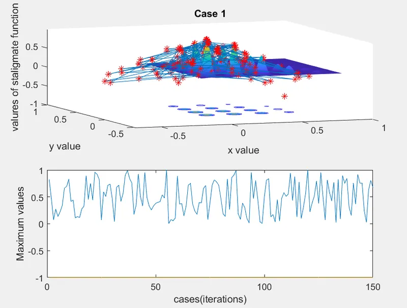
- In this first case giving 150 itrations to "ga" and not giving any initial and final points. so we get a large number of values
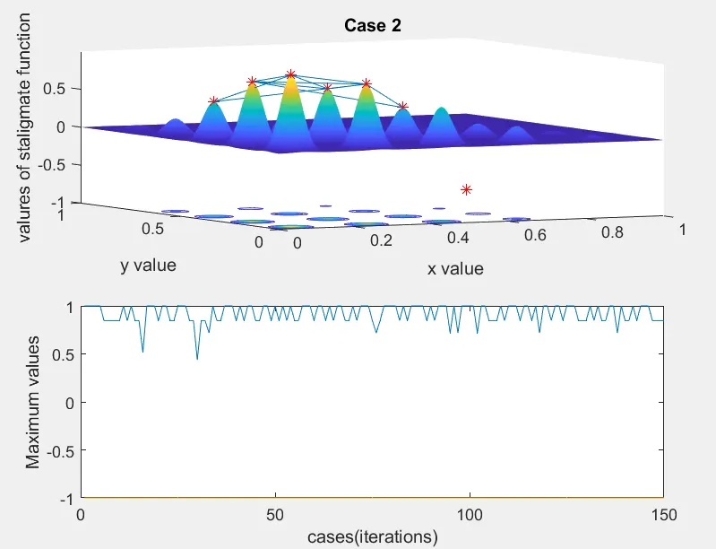
- At second case we provide limiting values then we get more acurate values we need
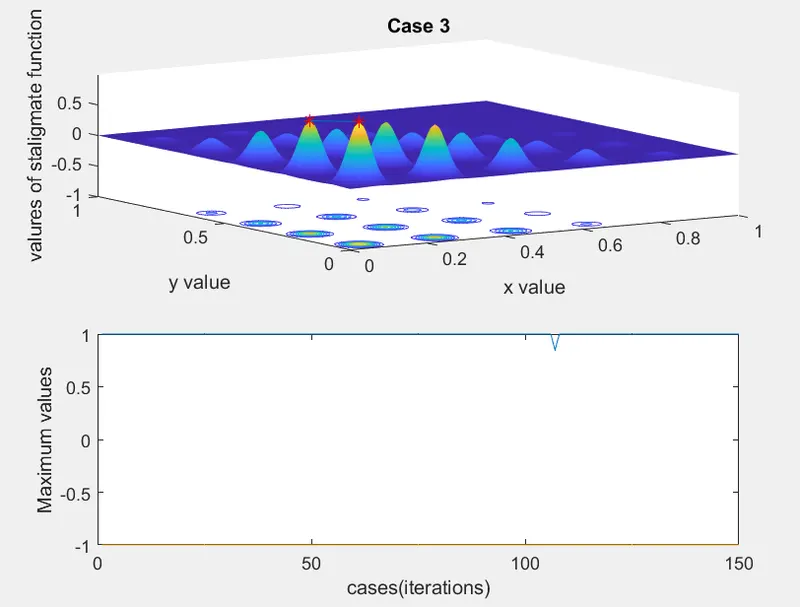
- In the third case we change options and increase the population size into 300 and so that we get more acurate results.
Reference:
- An Article by Musatafa Abbas Albadr, Sabrina Tiun, Masri Ayob and Fahad AL-Dhief. "Genetic Algorithm Based on Natural Selection Theory for Optimization Problems".
ga