Project 2 - Rankine cycle Simulator

Objective

• Understand the concept of Rankine cycle
• Create a Rankine Cycle Simulator using MATLAB.
• Your code should calculate the state points of the Rankine Cycle.
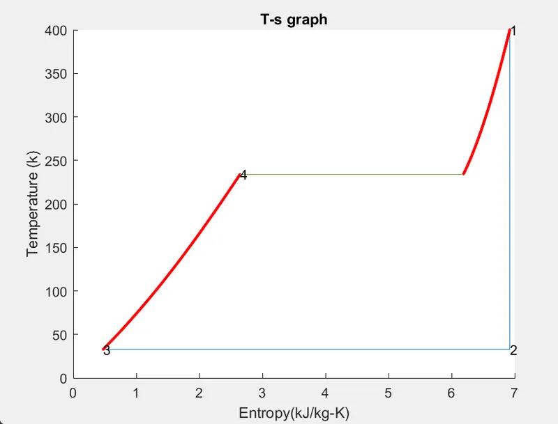
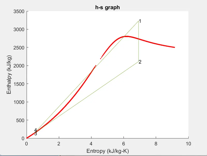
• Then, plot the corresponding T-s and h-s plots for the given set of inputs.

Rankine cycle

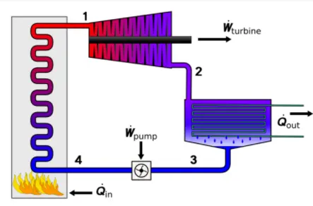
The working fluid is compressed from low to high pressure (Step 3-4). At this stage, the pump requires little input energy because the fluid is a liquid. The high-pressure liquid enters a boiler, where it is heated at constant pressure to the compressed liquid (Step 4-1) and two-phase (i.e., water and steam) mixture. The steam is then passed through the superheaters, where it superheated. The steam is then expanded through a turbine to generate power (Step 1-2). The expanded vapor, which is decreased in temperature and pressure, enters a condenser, where it is condensed at a constant pressure and temperature to become a saturated liquid and the unavailable heat is rejected to the atmospheric sink (Step 2-3).

The thermodynamic efficiency depends on the temperatures at which heat addition and rejection occur:

CODE

clear 
close
clc

% input values

P1 = 30;
T1 = 400;
P2 = .05;
t  = linspace(0,400,800);

% state 1

h1    = XSteam('h_PT',P1, T1); 
s1    = XSteam('s_PT',P1, T1);
hl1   = XSteam('hL_p',P1);
hg1   = XSteam('hV_p', P1);
sl1   = XSteam('sl_p',P1);
sg1   = XSteam('sV_p',P1);
Tsat1 = XSteam('Tsat_p',P1);


disp('At state point 1: ')
disp(' ')
fprintf('P1 = %.2f bar \n',P1)
fprintf('s1 = %.2f kJ/kgk \n',s1)
fprintf('T1 = %.2fDegree celcius \n', T1)
fprintf('h1 = %.2f kJ/kg \n', h1)
disp(' ')


% At state point 2

s2    = s1;
s12   = XSteam('sL_p',P2); 
sg2   = XSteam('sV_p',P2);
d     =(s2-s12)/(sg2-s12);
h12   = XSteam('hL_p',P2);
hg2   = XSteam('hV_p',P2); 
h2    = h12 + d*(hg2-h12);
T2    = XSteam('T_ph', P2, h2); 
Tsat2 = XSteam('Tsat_p',P2);


disp('At state point 2: ')
disp(' ')
fprintf('P2 = %.2fbar \n',P2) 
fprintf('T2 = %.2fDegree celcius \n',T2)
fprintf('h2 = %.2fkJ/kg \n', h2) 
fprintf('s2 = %.2fkJ/kgk \n', s2)
disp(' ')


% At state 3

h3 = h12;
s3 = s12;
P3 = P2;
T3 = T2;


disp('At state point 3: ')
disp(' ')
fprintf('P3 = %.2fbar \n',P3)
fprintf('T3 = %.2fDegree celcius \n', T3)
fprintf('h3 = %.2fkJ/kg \n', h3) 
fprintf('s3 = %.2fkJ/kgk \n',s3)
disp(' ')


% At state 4

s4 = s3; 
P4 = P1;
h4 = XSteam('h_ps',P4, s4);
T4 = XSteam('T_ps',P4, s4);


disp('At state point 4: ')
disp(' ')
fprintf('P4 = %.2fbar \n', P4)
fprintf('T4 = %.2fDegree celcius \n', T4)
fprintf('h4 = %.2fkJ/kg \n',h4)
fprintf('s4= %.2fkJ/kgk \n', s4)
disp(' ')


% Work done and efficiency

W_turbine = h1-h2;

W_pump    = h4-h3;

W_net     = W_turbine - W_pump;

therm_eff = (1-((h2-h3)/(h1-h4)))*100;

back_wr   = W_pump/W_turbine;


fprintf('Work done by turbine = %.2fkJ/kg \n', W_turbine)
fprintf('Work done by pump = %.2fkJ/kg \n', W_pump)
fprintf('Net work done = %.2fkJ/kg \n', W_net)
fprintf('Thermal efficiency = %.2f%% \n', therm_eff)
fprintf('Back-work ratio = %.4f \n', back_wr)
disp(' ')



figure(1)

hold on

plot([s1 s2 s3], [T1 T2 T3])

n = linspace (T1,T2,500);

for i=1:length(n)
    plot (XSteam('s_pT',P1, n(i)), n(i),'r.')
end

 plot([sl1 sg1], [Tsat1 Tsat1])


text (s1, T1, '1')
text (s2, T2, '2')
text (s3, T3, '3')
text (sl1, Tsat1, '4')
xlabel('Entropy(kJ/kg-K)')
ylabel('Temperature (k)')
title('T-s graph')



figure(2)

hold on

for i=1:length(t)
plot (XSteam('sL_T',t(i)), XSteam ('hL_T',t(i)), 'r.') 
plot (XSteam('sV_T',t(i)), XSteam('hV_T',t(i)), 'r.')
end

plot([s1 s2 s3 s4 s1], [h1 h2 h3 h4 h1]) 
text (s1, h1, '1')
text (s2, h2, '2') 
text (s3, h3, '3')
text (s4, h4+90,'4')
xlabel('Entropy (kJ/kg-K)')
ylabel('Enthalpy (kJ/kg)')
title('h-s graph')

Code explanation

• First of all we requered to save Xsteam functions. That Xsteam is given with the question.
• Then "clear , close , clc" for clear all the unwanted history.
• Provide all given inputs.
• Then calculated all the state point values.
• At the same time print the required state point values in the command window using "fprintf".
• Then find thermal efficiency, work done, back work and printed output in command window.
• Then we want to plot T-S and H-S graph. for creating the required two plots we use each state point values and that values give streight lines and for curved values we use for loop. And also give xlabel , ylabel , title of the graph.
• use "test" command for showing the state point's

Output

• In command window

At state point 1: 
 
P1 = 30.00 bar 
s1 = 6.92 kJ/kgk 
T1 = 400.00Degree celcius 
h1 = 3231.57 kJ/kg 
 
At state point 2: 
 
P2 = 0.05bar 
T2 = 32.88Degree celcius 
h2 = 2110.71kJ/kg 
s2 = 6.92kJ/kgk 
 
At state point 3: 
 
P3 = 0.05bar 
T3 = 32.88Degree celcius 
h3 = 137.77kJ/kg 
s3 = 0.48kJ/kgk 
 
At state point 4: 
 
P4 = 30.00bar 
T4 = 32.95Degree celcius 
h4 = 140.76kJ/kg 
s4= 0.48kJ/kgk 
 
Work done by turbine = 1120.86kJ/kg 
Work done by pump = 3.00kJ/kg 
Net work done = 1117.87kJ/kg 
Thermal efficiency = 36.17% 
Back-work ratio = 0.0027 
 

We finded out all the required state point values, work done, back work ratio.

• Graphs
• 
•