Week 4.1 - Genetic Algorithm

Theory:-

Genetic Algorithm is a method that workson the principal of Darwin's Theory of natural selection i.e- Survival of the fittest.

There are five phases that are considered in genetic algorithm:-

1) Initial function

2) Fitness function

3) Selection

4)Crossover

5)Mutation

*ga function only gives minimum value.

[x,fval] = ga(function,no_of_variables,A,b,Aeq,beq,lb,ub,nonlcon,Intcon,options).

where,

1. x = optimum variables

2. no_of_variables = Number of variables, specified as a positive integers

3. A,b = linear Inequalities constraints

4. Aeq,beq = Linear equality constraints

5. lb,ub = Lower bounds , Upper Bounds Respectively

6. nonlcon = Use of non-linear constraints

7. IntCon = To get solution in integer

8. Options = Minimize with non default options

CODE:-

function [F] = stalagmite(input_vector)
x = input_vector(1);
y = input_vector(2);

f1_x = (sin(5.1*pi*x+0.5)).^6;
f1_y = (sin(5.1*pi*y+0.5)).^6;
f2_x = exp(-4*log(2)*((x-0.0667).^2)/0.64);
f2_y = exp(-4*log(2)*((y-0.0667).^2)/0.64);
[F] = -(f1_x.*f1_y.*f2_x.*f2_y);
end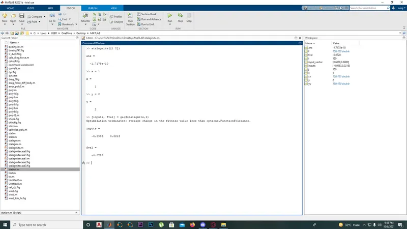

Genetic_algorithm:-

clear all
close all
clc

% Defining our search space
x = linspace(0,0.6,150);
y = linspace(0,0.6,150);
% Creating a 2Dimensional mesh
[xx,yy] = meshgrid(x,y);

% Evaluating the stalagmite function
for i = 1:length(xx)
    for j = 1:length(yy)
        input_vector(1) = xx(i,j);
        input_vector(2) = yy(i,j);
        f(i,j) = stalagmite(input_vector);
    end
end

%Surface(xx,yy,f)
figure (1)
surf(xx,yy,-f)
shading interp

xlabel ('x value')
ylabel('y value')
title('Initial Stalagmite')
colorbar

[inputs, fval] = ga(@stalagmite, 2) 

Genetic_algorithm_1:-

clear all
close all
clc

% Defining our search space
x = linspace(0,0.6,150);
y = linspace(0,0.6,150);
% Creating a 2Dimensional mesh
[xx,yy] = meshgrid(x,y);

% Evaluating the stalagmite function
for i = 1:length(xx)
    for j = 1:length(yy)
        input_vector(1) = xx(i,j);
        input_vector(2) = yy(i,j);
        f(i,j) = stalagmite(input_vector);
    end
end
tic
%Study1 - Statical behaviour
n = 50;
for i = 1:n
    [inputs, fopt(i)] = ga(@stalagmite,30);
    xopt(i) = inputs(1);
    yopt(i) = inputs(2);
end
study1_time = toc
F = -f;
figure (1)
subplot(2,1,1)
hold on
surfc(x, y, F)
shading interp
plot3(xopt,yopt,-fopt,'marker','o','MarkerSize',5,'MarkerFaceColor','r')
title('Unbouded inputs')
xlabel('x')
ylabel('y')
zlabel('f')
subplot(2,1,2)
plot(-fopt)
xlabel('Iterations')
ylabel('Function maximum')
  

Genetic_algorithm_2:-

clear all
close all
clc

% Defining our search space
x = linspace(0,0.6,150);
y = linspace(0,0.6,150);
% Creating a 2Dimensional mesh
[xx,yy] = meshgrid(x,y);

% Evaluating the stalagmite function
for i = 1:length(xx)
    for j = 1:length(yy)
        input_vector(1) = xx(i,j);
        input_vector(2) = yy(i,j);
        f(i,j) = stalagmite(input_vector);
    end
end

%Study2 - Statical behaviour with upper and lower bounds
options = optimoptions('ga','PopulationSize',50);
tic
n = 50;
for i = 1:n
    [inputs, fopt(i)] = ga(@stalagmite,2,[],[],[],[],[0;0],[0.6;0.6]);
    xopt(i) = inputs(1);
    yopt(i) = inputs(2);
end
study2_time = toc
F = -f;
figure (2)
subplot(2,1,1)
hold on
surfc(x, y, F)
shading interp
plot3(xopt,yopt,-fopt,'marker','o','MarkerSize',5,'MarkerFaceColor','r')
title('Unbouded inputs')
xlabel('x')
ylabel('y')
zlabel('f')
subplot(2,1,2)
plot(-fopt)
xlabel('Iterations')
ylabel('Function maximum')
  

Genetic_algorithm_3:-

clear all
close all
clc

% Defining our search space
x = linspace(0,0.6,150);
y = linspace(0,0.6,150);
% Creating a 2Dimensional mesh
[xx,yy] = meshgrid(x,y);

% Evaluating the stalagmite function
for i = 1:length(xx)
    for j = 1:length(yy)
        input_vector(1) = xx(i,j);
        input_vector(2) = yy(i,j);
        f(i,j) = stalagmite(input_vector);
    end
end

%Study3 - Increasing GA iteration
options = optimoptions('ga','PopulationSize',200);
tic
n = 50;
for i = 1:n
    [inputs, fopt(i)] = ga(@stalagmite,2,[],[],[],[],[0;0],[0.6;0.6],[],[],options);
    xopt(i) = inputs(1);
    yopt(i) = inputs(2);
end
study3_time = toc
F = -f;
figure (2)
subplot(2,1,1)
hold on
surfc(x, y, F)
shading interp
plot3(xopt,yopt,-fopt,'marker','o','MarkerSize',5,'MarkerFaceColor','r')
title('Unbouded inputs')
xlabel('x')
ylabel('y')
zlabel('f')
subplot(2,1,2)
plot(-fopt)
axis([0 50 0 1.5]);
xlabel('Iterations')
ylabel('Function maximum')
FMAX = -min(fopt);
X = mean(xopt);
Y = mean(yopt);