Week 4.1 - Genetic Algorithm

Aim

Write a code in MATLAB to optimise the stalagmite function and find the global maxima of the function.

Introduction

How Genetic Algorithm Works?

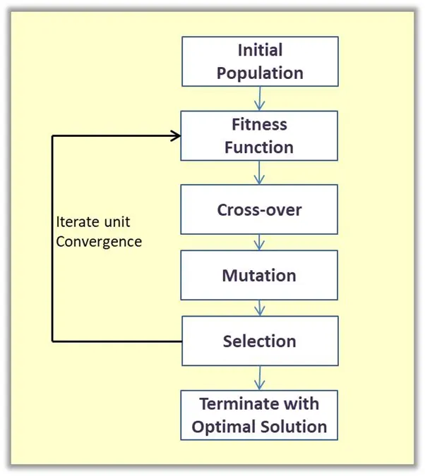
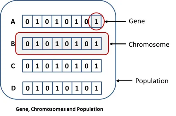
Genetic Algorithm works by the process of natural selection. It starts from an initial, maybe random population (which represent a pool of all possible solutions to a problem). Then these population undergoes several processed such as Selection, Cross-Over and Mutation and finally produces the best results (optimal solution) at the end of the process.

Overview of the gene, chromosome, population

4. Phases in Genetic Algorithm

Genetic Algorithm proceeds from an initial population through several phases till the termination when the optimal solution have been deduced. Let’s now examine the different phases of Genetic algorithm.

1. Initial Population

This is the first phase of the process where an initial population is selected. The initial population is simply a set of individuals which are potential solution to the problem we want to solve. It could actually be made of of thousands or even hundreds of thousands of individuals that may have been randomly selected or selected based on some specified criteria. The two methods of initializing the population are summarized as:

2.Fitness Function Definition

This phase could also be regarded as part of the Initial phase (Initial Population) and it could also be part of the Selection phase. This is a way of specifying the criteria for the ‘goodness’ of a given solution compared to others and to the problem being solved. Based on the fitness, members of the population are separated into two parts: those that are fit enough to be selected into the next generation and those that would be dropped.

One approach to this is to have a fitness score for each individual in the population. So when this score is passed into the fitness function, it returns either 1(pass) or 0 (fail).

3.Cross-Over

Cross-over is the most noteworthy of the phases of genetic algorithm. This is also called recombination. It is a genetic operator that determines what information is passed from the two parents to the new offspring. This is illustrated below in Figure

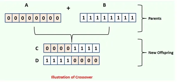
Cross-over point is the point in within the genes of the parents at which the cross-over occurs.

4.Mutation

Mutation is a random change in the chromosome of the new offspring. This change occurs with a little probability. The benefit of this phase is that if tends to prevent the algorithm from converging in a local minimum. To do this, a mutation rate is carefully chosen. This is illustrated in Figure below

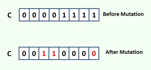
5.Termination

After a number of iterations through the phases of the algorithm, the process terminates based on certain defined termination criteria. At this stage the optimal solution is reached.

Explanation of the code

Sub code

function [f]=stalagmite(input_vector)

x=input_vector(1);

y=input_vector(2);

Input vector is divided into 2 variables x,y because only then we use ga (generic algorithm ) to find global minima

f1=(sin(5.1*pi*x+0.5))^6;

f2=(sin(5.1*pi*y+0.5))^6;

f3=exp(-4*log(2)*((x-0.0667)^2)/0.64);

f4=exp(-4*log(2)*((y-0.0667)^2)/0.64);

f=-(f1*f2*f3*f4);

end

to create stalagmite the above codes are used.

Main code

• clear all (This clears your workspace) ,
• close all(closes all figures) and
• clc (clears the command window).

Generate linearly spaced vector

x=linspace(0,0.6,150);

y=linspace(0,0.6,150);

Transforms the domain specified by vectors x and y into arrays X and Y, which can be used to evaluate functions of two variables and three-dimensional mesh/surface plots.

[xx yy]=meshgrid(x ,y);

After calling the the fuction the values of input_vectors(1) and input_vectors(2) is assigned as per the order of (i, j)

f(i,j)=stalagmite(input_vector);

Nested for loop is used to assign values to i and j as per the order of iteration and storing the data to the variables input_vectors(1) and input_vectors(2).

for i=1:length(xx);

for j=1:length(yy);

input_vector(1)=xx(i,j);

input_vector(2)=yy(i,j);

f(i,j)=stalagmite(input_vector);

end

end

Tic toc is used to measure the amount of time MATLAB takes to complete one or more operations, and displays the time in seconds.

In here tic toc is used to calculate the time required to finish the for loop from 1 to num_cases.

ga is used to identify the global minimum value from the stalagmite

(-f) we introduce negative sign in order to flip the stalagmite

(-fopt) we introduce negative sign in the code in order to get the global maximum

INPUTS- it is the array where the selected optimum variables from xopt, yopt is stored.

fopt(i)- it is the array were all the selected optimum variables of x, y are stored according to the sequence

ga(@stalagmite,2) –(ga)genetic algorithm to find the global minima from the stalagmite and 2 indicates the x and y variable

xopt- optimum values if x gets stored in xopt

yopt- optimum values of y gets stored in yopt

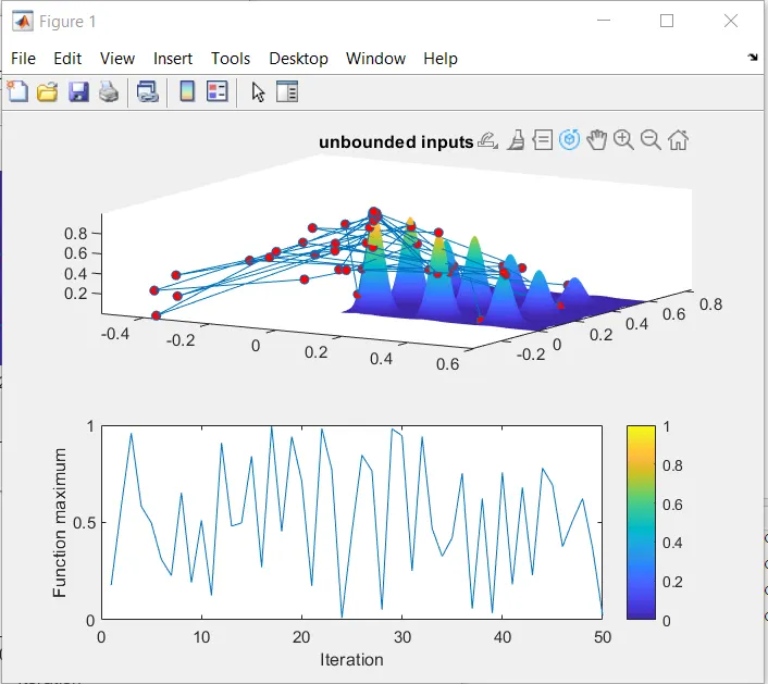
In case 1 we have not provided with the upper and the lower bounds

tic

%study 1 statistical behavior

num_cases=50;

for i=1:num_cases;

[INPUTS , fopt(i)]=ga(@stalagmite,2)

xopt(i)=INPUTS(1);

yopt(i)=INPUTS(2);

end

study1_time=toc

ploting the figure one

in figure1 sub dividing using subplot

surf command is used to plat a surface plot of the values stored in f

shading interp is used to plot a smooth surface

plot3 is used for 3D plot

plot is used for 2d plot

figure(1)

subplot(2,1,1)

hold on

surfc(xx, yy ,-f)

shading interp

plot3(xopt ,yopt ,-fopt,'marker','o','markersize',5,'markerfacecolor','r')

title('unbounded inputs')

subplot(2,1,2)

plot(-fopt)

colorbar

xlabel('Iteration')

ylabel('Function maximum')

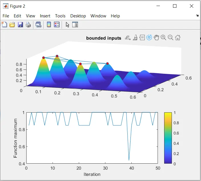
Everything is as same as the previous case with the only difference is to set upper and lower bounds

ga(@stalagmite,2,[],[],[],[],[0;0],[1;1]); -the bounds set so the selected variables will be within the limit that is 0 to 1 in both x and y axis and wont be outside the bounds as the first case(by comparing the figure 1 and 2 it will give a better idea)

%study 2 -statistal behavior -with upper and lower bounds

tic

for i=1:num_cases;

[INPUTS , fopt(i)]=ga(@stalagmite,2,[],[],[],[],[0;0],[1;1]);

xopt(i)=INPUTS(1);

yopt(i)=INPUTS(2);

end

study2_time =toc

figure(2)

subplot(2,1,1)

hold on

surfc(xx, yy ,-f)

shading interp

plot3(xopt ,yopt ,-fopt,'marker','o','markersize',5,'markerfacecolor','r')

title('bounded inputs')

subplot(2,1,2)

plot(-fopt)

colorbar

xlabel('Iteration')

ylabel('Function maximum')

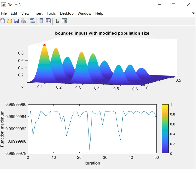
The default population size used by ga is 50 when the number of decision variables is less than 5, and 200 otherwise.

In this case the only change made is increasing the population size to get 400 vaules using options syntax in order to get best value.

%study 3 statistal behavior -with increasing ga iteration

options = optimoptions('ga','PopulationSize',400)

tic

for i=1:num_cases;

[INPUTS , fopt(i)]=ga(@stalagmite,2,[],[],[],[],[0;0],[1;1],[],[],options);

xopt(i)=INPUTS(1);

yopt(i)=INPUTS(2);

end

study3_time =toc

figure(3)

subplot(2,1,1)

hold on

surfc(xx, yy ,-f)

shading interp

plot3(xopt ,yopt ,-fopt,'marker','o','markersize',5,'markerfacecolor','r')

title('bounded inputs with modified population size')

subplot(2,1,2)

plot(-fopt)

colorbar

xlabel('Iteration')

ylabel('Function maximum')

syntax for ga

if certian variables are not present then we provide with the square brackets[]

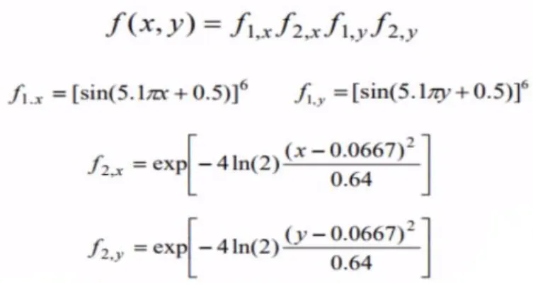
code

function [f]=stalagmite(input_vector)

x=input_vector(1);
y=input_vector(2);
f1=(sin(5.1*pi*x+0.5))^6;
f2=(sin(5.1*pi*y+0.5))^6;
f3=exp(-4*log(2)*((x-0.0667)^2)/0.64);
f4=exp(-4*log(2)*((y-0.0667)^2)/0.64);
f=-(f1*f2*f3*f4);
end

clear all
close all
clc

x=linspace(0,0.6,150);
y=linspace(0,0.6,150);

[xx yy]=meshgrid(x ,y);


for i =1:length(xx);
for j=1:length(yy);
    input_vector(1)=xx(i,j);
    input_vector(2)=yy(i,j);
   f(i,j)=stalagmite(input_vector);
end
end


tic
%study 1 statistical behavior
num_cases=50;
for i=1:num_cases;

   [INPUTS , fopt(i)]=ga(@stalagmite,2)
    xopt(i)=INPUTS(1);
    yopt(i)=INPUTS(2);
end
study1_time=toc

figure(1)
subplot(2,1,1)
hold on
surfc(xx, yy ,-f)
shading interp
plot3(xopt ,yopt ,-fopt,'marker','o','markersize',5,'markerfacecolor','r')
title('unbounded inputs')
subplot(2,1,2)
plot(-fopt)
colorbar
xlabel('Iteration')
ylabel('Function maximum')

%study 2 -statistal behavior with upper and lower bounds
tic

    for i=1:num_cases;

   [INPUTS , fopt(i)]=ga(@stalagmite,2,[],[],[],[],[0;0],[1;1]);
    xopt(i)=INPUTS(1);
    yopt(i)=INPUTS(2);
    end
   
   study2_time =toc
figure(2)
subplot(2,1,1)
hold on
surfc(xx, yy ,-f)
shading interp
plot3(xopt ,yopt ,-fopt,'marker','o','markersize',5,'markerfacecolor','r')
title('bounded inputs')
subplot(2,1,2)
plot(-fopt)
colorbar
xlabel('Iteration')
ylabel('Function maximum')

%study 3 statistal behavior increasing GA iteration 
options = optimoptions('ga','PopulationSize',400)
tic

    for i=1:num_cases;

   [INPUTS , fopt(i)]=ga(@stalagmite,2,[],[],[],[],[0;0],[1;1],[],[],options);
    xopt(i)=INPUTS(1);
    yopt(i)=INPUTS(2);
    end
    study3_time =toc
figure(3)
subplot(2,1,1)
hold on
surfc(xx, yy ,-f)
shading interp
plot3(xopt ,yopt ,-fopt,'marker','o','markersize',5,'markerfacecolor','r')
title('bounded inputs with modified population size')
subplot(2,1,2)
plot(-fopt)
colorbar
xlabel('Iteration')
ylabel('Function maximum')

Result

case 1

Unbounded inputs

case2

Bounded inputs in order to have the values with the range

case3

Bounded inputs with the bounds and modified population size to get the best value

Reference

https://www.mathworks.com/discovery/genetic-algorithm.html

https://youtu.be/f0bGSPo5aJk