Week 4.1 - Genetic Algorithm

AIM:

To write a code in matlab and optimise the stalagmite function and to evaluate the global maxima of the function.

INTRODUCTION:

Stalagmite:

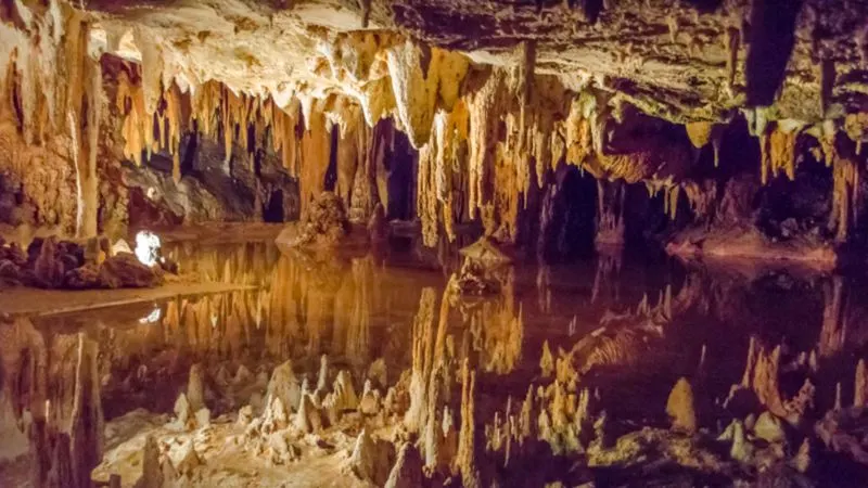
A stalagmite is an upward growing mound of mineral deposits that have precipitated from water dripping onto the floor of a cave. Most stalgamite have rounded or flattened tips.There are many other form of mineral found in the cave.

Stalactite:

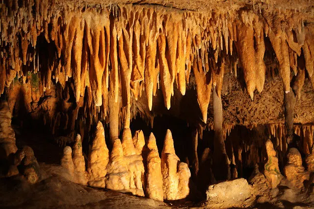
A Stalactite is a mineral formation that hangs from the ceiling of the caves, hot springs, man made structures such as bridges and sculptures. Any material that can be soluble and can be deposited as a colloid or can be melted may form a stalactite.

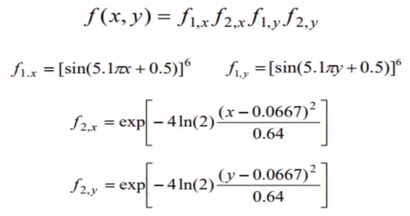
The Stalagmite function is defined below:

Optimization:

Maximing or minimizing a function relative to some set often representing a range of choices available in a certain situation. The function allows comparison of the different choices for determining which might be best.

Common applications: Minimalcost;Maximum profit

Generic Algorithm:

Genetic algorith is a search heuristic that is inspired by charles darwins theory of natural evolution.This algorithm reflects the process of natural selection where the fittest individuals are selected for natural selection in order to prduce offspring of the next generation.

Genetic algorithm optimization starts with population initialization

Population is the number of sample data points taken to perfor the genetic algorithm operation. These sample data points undergo the following three steps

Selection:

In this step the parents are selected from the sample data points , the main objective of the selection process is to select the highly fit individuals.

Example: Roulette wheel selection

Cross over:

It is the process of taking two parents solution and producing the child from them

Mutation:

Mutation is carried out to maintain the genetic diversity of one generation of population of chromosomes to the next.If mutation is not performed the chromosomes looks so similar to eacg other, convergence takes place soon and results in local minima .

Examplae :swap mutation

Objectives:

• A code in matlab to optimize the stalagmite function
• To find the global maxima of the function
• To run the program for three alternate cases

Main Program:

%Start of the program

close all
clear all
clc

%Assigning initial values
x = linspace(0,0.6,80);
y = linspace(0,0.6,80);
limit = 50;

%Mesh grid function
[xx yy] = meshgrid(x,y);

%Nested for loop for inputs
for i = 1:length(xx)
  for  j = 1:length(yy)
    input_vector(1) = xx(i,j);
    input_vector(2) = yy(i,j);
    f(i,j) = stalagmite_fun(input_vector);
  end
end

tic
for i = 1:limit
    
    [input,fval(i)] = ga(@stalagmite_fun,2);
    x_out(i) = input(1);
    y_out(i) = input(2);
    
end
 
%Case1: Unbounded
case_time_1 = toc

figure(1)
subplot(2 ,1, 1)
surf(xx, yy ,-f)
xlabel('x')
ylabel('y')
title('Case1(Unbounded)','color','k')
shading interp
hold on;
 plot3(x_out,y_out,-fval,'marker','o','markersize',6,'markerfacecolor','r')
subplot(2 ,1 ,2)
plot(-fval);
xlabel('no of iterations')
ylabel('max function value')

%Case2: With boundbox
 tic
 for i = 1:limit
     
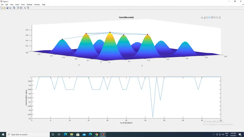
     [input,fval(i)] = ga(@stalagmite_fun,2,[], [], [], [],[0;0],[0.6;0.6]);
     x_out(i) = input(1);
     y_out(i) = input(2);
     
 end
 
 case_time_2 = toc;
 
figure(2)
subplot(2 ,1, 1)
hold on
surfc(xx, yy ,-f)
xlabel('x')
ylabel('y')
title('Case2(Bounded)','color','k')
shading interp
hold on;
plot3(x_out,y_out,-fval,'marker','o','markersize',6,'markerfacecolor','r')
subplot(2 ,1 ,2)
plot(-fval)
xlabel('no of iterations')
ylabel('max function value')

%Case 3: Bounded with population size
options = optimoptions('ga');
options = optimoptions(options,'populationsize',100)

 tic
 for i = 1:limit
     
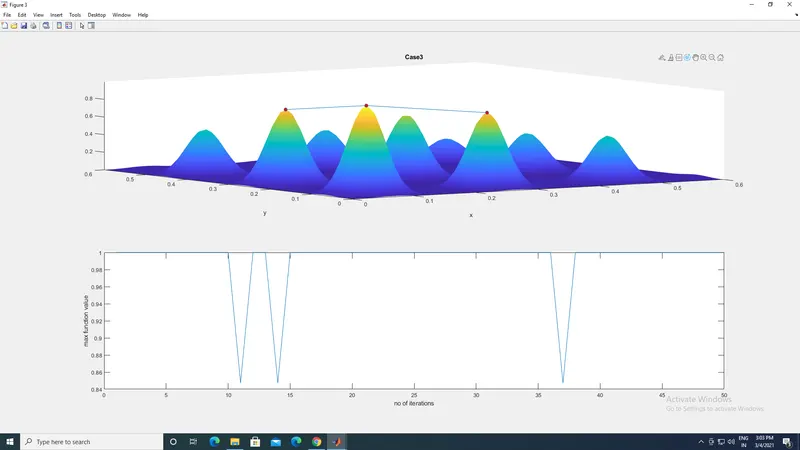
     [input,fval(i)] = ga(@stalagmite_fun,2,[], [], [], [],[0;0],[0.6;0.6],[],[],options);
     x_out(i) = input(1);
     y_out(i) = input(2);
     
 end
 
 case_time_3 = toc;
 
figure(3)
subplot(2 ,1, 1)
hold on
surfc(xx, yy ,-f)
xlabel('x')
ylabel('y')
title('Case3','color','k')
shading interp
hold on
plot3(x_out,y_out,-fval,'marker','o','markersize',6,'markerfacecolor','r')
subplot(2 ,1 ,2)
plot(-fval)
xlabel('no of iterations')
ylabel('max function value')


%Case 4: Bounded with increased population size
options = optimoptions('ga');
options = optimoptions(options,'populationsize',300)

 tic
 for i = 1:limit
     
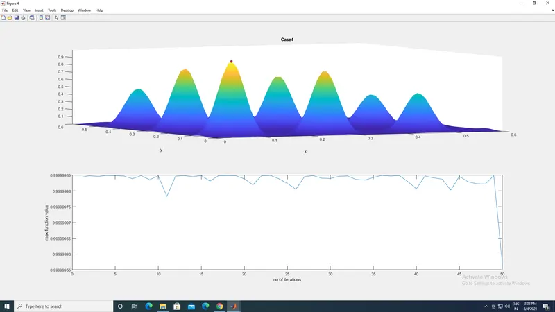
     [input,fval(i)] = ga(@stalagmite_fun,2,[], [], [], [],[0;0],[0.1;0.1],[],[],options);
     x_out(i) = input(1);
     y_out(i) = input(2);
     
 end
 
 case_time_4 = toc;
 
figure(4)
subplot(2 ,1, 1)
hold on;
surfc(xx, yy ,-f)
xlabel('x')
ylabel('y')
title('Case4','color','k')
shading interp
hold on;
plot3(x_out,y_out,-fval,'marker','o','markersize',6,'markerfacecolor','r')
subplot(2 ,1 ,2)       


plot(-fval)
xlabel('no of iterations')
ylabel('max function value')

%Displaying the value of x and y for max value of function
display(input)

%End of program

Stalagmite function program:

function[f1] = stalagmite_fun(input_vector)

f1x = (sin(5.1*pi*input_vector(1)+0.5))^6;
f1y =(sin(5.1*pi*input_vector(2)+0.5))^6;

f2x = exp((-4*log(2))*(input_vector(1)-0.0667)^2/0.64);
f2y = exp((-4*log(2))*(input_vector(2)-0.0667)^2/0.64);
f1 = -f1x *f1y *f2x *f2y;

end

Output graphs:

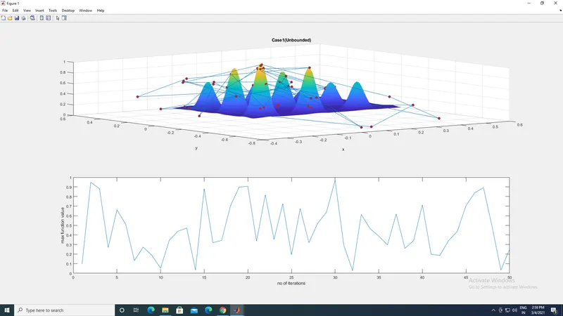
CASE 1(Unbounded):

CASE 2(Bounded):

CASE 3:

CASE 4:

Program Explanation:

So in start of the program we use close all ,clear all, clc to initialize the program . Then a range of values are created for x and y with a limit of 50 from 0 to 0.6. An array is created by using the mesh grid function for xx and yy. Nested loop is used to store the values of i and j in array input vector 1 and 2 . Then the stalagmite function is used having the inputs as input vector. ga command is used to find the values that can be used for function value by specifying the no of variables as 2 . Tic toc command is used to note the time limit for each graph values of different cases.Sub plot is used to give the coordinates for the lines to join to make the cases perfect. Here x is labelled as 'no of iterations' and y is labelled as 'max value function' . Then for case 2 w eare using a bound box to create a different case. xoutput and y output are used as output return values for the given inputs of 1 and 2.Then the cases are written for different subplots and values .Then finally the graph is plotted using the plot command giving the three cases results. On the other extension we have written the stalagmite function.

Errors:

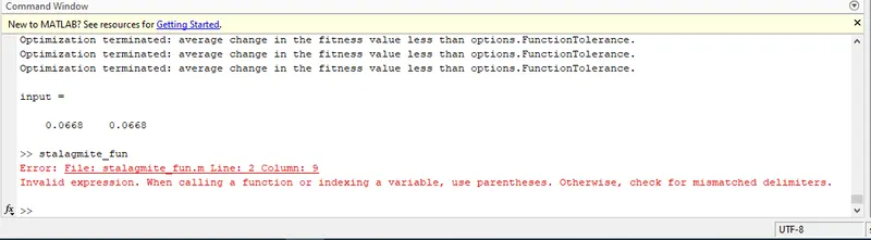
Here in the main program I have used parenthesis, instead of square brackets.

Conclusion:

Thus I have written a program in matalb to optimize the stalagmite function and to find the global maximum of the function.