Week 3 - Solving second order ODEs

INTRODUCTION:

Simple Pendulum:

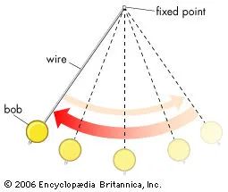
A point mass attached to a light inextensible string and suspended from fixed support is called a simple pendulum. The vertical line passing through the fixed support is the mean position of a simple pendulum.The vertical distance between the point of suspension and the centre of mass of the suspended body (when it is in mean position) is called the length of the simple pendulum denoted by L.The simple pendulum comprises of a small bob of mass ‘m’ suspended by a thin string secured to a platform at its upper end of length L.

AIM:
   To solve the second order ODEs using Matlab program

FORMULA:

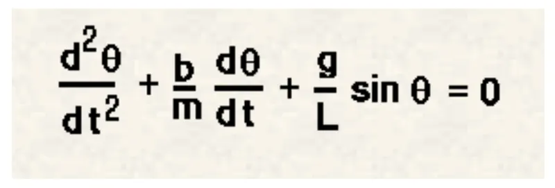
Where

m - mass of the bob

g - gravity in m/s

`theta`- angle made by the string with the fixed part

L - lenght of the string

b - damping coefficient

OBJECTIVES:

• To solve the second order ODE using Matlab program.
• To create an animation projecting the motion of the pendulum.

FUNCTON OF THE PROGRAM:

function [dtheta_dt] = ode_func(t,theta,b,g,l,m)

theta1 = theta(1)
theta2 = theta(2)
dtheta1_dt = theta2;
dtheta2_dt = -(b/m)*theta2 - (g/l)*sin(theta1);
dtheta_dt = [dtheta1_dt;dtheta2_dt];

end

MAIN PROGRAM:

clear all
close all
clc

b = 0.05;
g = 9.81;
l = 1;
m = 1;

%Initial conditions
theta_0 = [0;3];

%timepoints
t_span = linspace(0,20,500);

% solve ode
[t,results] = ode45(@(t,theta) ode_func(t,theta,b,g,l,m),t_span,theta_0);

%plotting
plot(t,results(:,1))
hold on
plot(t,results(:,2))
xlabel('Plot')
ylabel('time')

theta = results(:,1);
c = 1;

for i = 1:length(theta)
    Theta = theta(i);
    
    %initial points
    x0 = 0;
    y0 = 0;
    
    %movement of pendulum
    x1 = l*sin(Theta);
    y1 = -l*cos(Theta);
    
    figure(2)
    %plotting string
    plot([x0 x1], [y0 y1],'color','g');
    hold on
    
    %plotting the bob
    plot(x1,y1,'o','markersize',20,'color','r');
    hold off
    
    axis([-1 1 -1.5 0 ]);
    pause(0.03);
    M(c) = getframe(gcf);
    c = c+1;
    
end

%Creating a movie
movie(M);
videofile = VideoWriter('pendulum.avi','Uncompressed avi')
open(videofile)
writeVideo(videofile,M)
close(videofile)

Pendulum simulation:

https://drive.google.com/file/d/1Mg0_R7Lhbl3mtjhNirZBVTQCsO9O7sRV/view?usp=sharing

Output Graph:

PROGRAM EXPLANATION:

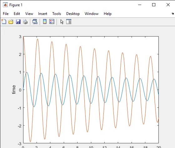
                 Here we first assign the given values for damping coefficient, mass of the ball, length of the string and damping coefficient. Then the initial dispacement for pendulum is '0' and the velocity at which the pendulum swings are '3' and the time is zero. ode45 function is used  to solve the 2nd order ode by using partial differential equation .So this gives the results in array of rows and columns in terms of velocity and displacement for every time variations. Then we are writing a separat ode function for assigning the values which are stored in ode 45.After calling the required function we are making some adjustements to the core values. Then we are using the plot command to plot the values of displacement and velocity. Then we are labelling the plot along x axis and time along y axis. Initial dispacement values for the pendulum is given as 0. Movement of the pendulum is written as using sin and cos values. Then we are plotting the lenght of the string and the bob. We are specifying the color of the bob and the veloity at which the string moves. Axis of the grapg is specified to project the limits. Getframe command is used to receive the graph values in frames to get some clarity of the movement of the pendulum. Pause command is used to pause the frames that is ongoing on the graph. The array M is used for storing the video file,videowriter is used to store the required file in avi and compress them in a folder. Finally write video is used to write trhe video and it is saved in that particular file. The animation of the pendulum is shown along with the veloity/displacement graph. 

Errors:

Error explanation:

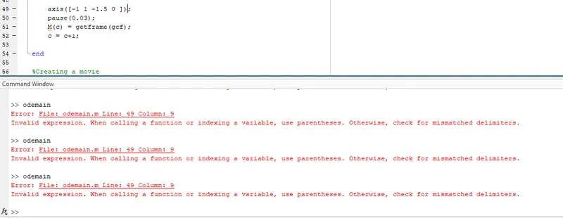
Here the error is I have used the parenthesis outside the array square brackets which is invalid in matlab.So here I should have used the parenthesis within the assigned values.

Conclusion:

Thus I have written a program to solve the ode problem and have used the values to simulate the motion of the pendulum.